
In the realm of unmanned aerial vehicles (UAVs), the ability to achieve precise temporal synchronization is a cornerstone for advanced collaborative missions. For small fixed-wing drones, which are often constrained by limited onboard computational resources, implementing a robust and efficient timed arrival control strategy is both challenging and essential. This article presents a detailed account of a control strategy I developed to enable small fixed-wing drones to arrive at a specified geographic location at a predetermined time and with a prescribed speed. The core idea revolves around constructing a virtual drone ideal motion model that serves as a real-time reference for guiding the actual drone’s flight path and velocity adjustments. Through this approach, the computational burden is minimized while maintaining high accuracy in meeting temporal constraints. I will elaborate on the mathematical formulation, the modeling of virtual drone kinematics, the handling of wind disturbances, and the simulation results that validate the effectiveness of the strategy.
1. Introduction to the Timed Arrival Problem
Timed arrival control is a fundamental capability for formation flight and coordinated task execution among multiple fixed-wing drones. In many applications, such as surveillance, search-and-rescue, or precision delivery, it is not sufficient for a drone to reach a waypoint; it must do so at a specified time and with a specific velocity to synchronize with other assets or to meet mission constraints. Traditional four-dimensional (4D) trajectory management techniques, widely used in civil aviation, rely on extensive computational resources for trajectory prediction and optimization. However, small fixed-wing drones typically have limited processing power, memory, and energy budgets, making direct adoption of these methods impractical. Hence, there is a need for a lightweight, yet effective, control strategy that can operate within the constraints of embedded flight computers.
My approach leverages a concept I call the “virtual drone ideal motion model.” This model is not a physical entity but a mathematical construct that describes the desired state (position, velocity, and time) of the drone along the predefined flight route. By continuously comparing the actual drone’s state with this virtual model, the control system generates corrective speed commands to minimize the deviation, thereby ensuring the actual drone “catches up” to or “slows down” to match the virtual drone’s schedule. This method avoids complex online trajectory optimization and instead relies on precomputed time-velocity tables that are updated only when significant changes occur (e.g., wind conditions or mission requirements). The strategy is designed to be computationally efficient, requiring only basic arithmetic operations and table lookups, which are well within the capabilities of typical autopilots used in small fixed-wing drones.
To set the stage, I make the following assumptions throughout this work:
- The drone is treated as a point mass, simplifying the dynamics and neglecting attitude effects on trajectory.
- The drone is equipped with sensors that provide reliable measurements of wind speed and direction, with negligible errors for the purpose of converting between indicated airspeed (IAS) and true airspeed (TAS).
- Except for moderate turbulence scenarios, the wind field is assumed to be constant (constant wind magnitude and direction) within each segment of the route, enabling algebraic derivation of speed-to-time relationships.
These assumptions allow me to focus on the core challenge of time control while keeping the mathematical treatment tractable. The strategy is nevertheless robust to non-constant wind conditions, as demonstrated later in simulation results.
2. The Virtual Drone Ideal Motion Model
The virtual drone ideal motion model is a predictive framework that encapsulates the desired trajectory in terms of time, position, and speed. It is built from the mission route data, which consists of a sequence of waypoints with associated required arrival times and speeds. Let us denote the waypoints as \(WP_0, WP_1, \ldots, WP_{tar}\), where \(WP_{tar}\) is the target waypoint with a specified arrival time \(T_{tar}\) and arrival speed \(V_{tar}\). For each segment between consecutive waypoints, we need to compute the time required to traverse that segment under ideal conditions (no wind, perfect tracking). The fundamental idea is to work backwards from the target waypoint: starting with the time needed for the final segment, we can compute the time at which the virtual drone should pass each preceding waypoint. This yields a table of “waypoint arrival times” that defines the virtual schedule.
Let \(L_i\) be the length of the segment from \(WP_i\) to \(WP_{i+1}\) (for \(i = 0, 1, \ldots, tar-1\)), and let \(V_i\) be the required speed at waypoint \(WP_i\) (typically the speed at the end of that segment). Under no-wind conditions, the true airspeed equals the ground speed, and the time for segment \(i\) is simply \(t_i = L_i / V_i\). However, when wind is present, the ground speed differs from true airspeed, and the calculation becomes more involved. I will address wind effects in a later section. For now, assume we can compute the segment times \(t_i\) using the appropriate formula. Then the arrival time at waypoint \(WP_i\) is given by:
$$
T_i = T_{tar} – \sum_{k=i}^{tar-1} t_k
$$
This produces a table of arrival times, as illustrated in Table 1.
| Waypoint | Segment Time (s) | Arrival Time (s) |
|---|---|---|
| WP₀ | t₀ | T₀ |
| WP₁ | t₁ | T₁ |
| … | … | … |
| WP_{n-1} | t_{n-1} | T_{n-1} |
| WP_{tar} | — | T_{tar} |
Once the arrival times are known, the instantaneous position of the virtual drone at any given real time \(T\) can be determined. Let \(\Delta t = T_{tar} – T\) be the remaining time to the target. Starting from the final segment, I check if \(\Delta t < t_{tar-1}\). If so, the virtual drone is currently in the last segment, and its distance from the target is \(\Delta L = \Delta t \times V_{tar}\). If \(\Delta t \ge t_{tar-1}\), I subtract \(t_{tar-1}\) from \(\Delta t\) and move to the previous segment, repeating until the segment containing the virtual drone is found. Mathematically, I find the smallest index \(m\) such that:
$$
\Delta t’ = T_{tar} – T – \sum_{k=m}^{tar-1} t_k < t_{m-1}
$$
Then the virtual drone is on segment \(WP_{m-1}\) to \(WP_m\), at a distance from \(WP_m\) equal to \(\Delta t’ \times V_m\). This geometric reasoning is illustrated conceptually in Figure 1 (see below). The virtual model thus provides a real-time reference for both position and velocity.
3. Handling Wind Disturbances
Wind is a critical factor affecting the accuracy of timed arrival for fixed-wing drones. The virtual drone model must account for wind to ensure that the schedule is realistic and achievable. I consider two types of wind conditions: constant wind fields (including headwind, tailwind, crosswind, and vertical wind) and moderate turbulence. For constant wind, the relationship between true airspeed (\(\mathbf{V}_t\)), ground speed (\(\mathbf{V}_d\)), and wind speed (\(\mathbf{V}_w\)) is:
$$
\mathbf{V}_d = \mathbf{V}_t + \mathbf{V}_w
$$
For straight-line segments, the drone’s ground speed must be aligned with the segment direction. Let \(\chi_d\) be the track angle (direction of the segment), and let \(\chi_w\) be the wind direction. Define the wind angle \(\chi_{WA} = \chi_d – \chi_w\) (or equivalently relative to the segment). Then the magnitude of ground speed can be derived from the law of cosines as:
$$
V_d = \sqrt{V_t^2 + V_w^2 + 2 V_t V_w \cos(\chi_{WA})}
$$
However, a more convenient form for computation is:
$$
V_d = V_t \left[ \sqrt{1 – \left(\frac{V_w}{V_t} \sin(\chi_{WA})\right)^2} + \frac{V_w}{V_t} \cos(\chi_{WA}) \right]
$$
This formula is valid for all angles. In the case of a pure headwind (\(\chi_{WA}=180^\circ\)), \(V_d = V_t – V_w\); for pure tailwind (\(\chi_{WA}=0^\circ\)), \(V_d = V_t + V_w\); for pure crosswind (\(\chi_{WA}=90^\circ\)), \(V_d = \sqrt{V_t^2 – V_w^2}\).
For curved segments (e.g., circular arcs), the direction of the segment changes continuously. To maintain computational efficiency on small fixed-wing drones, I discretize the arc into small straight-line segments. Let the arc have radius \(R\) and total turn angle \(\Delta \psi\). I divide \(\Delta \psi\) into \(N\) small increments \(\delta \psi\). For each increment, the local track angle changes, and the wind angle changes accordingly. The time to traverse each small segment is:
$$
\delta t_j = \frac{R \, \delta \psi}{V_t \left[ \sqrt{1 – \left(\frac{V_w}{V_t} \sin(\chi_{WA,j})\right)^2} + \frac{V_w}{V_t} \cos(\chi_{WA,j}) \right]}
$$
Summing over all increments gives the total segment time:
$$
t_i = \sum_{j=1}^{N} \delta t_j
$$
Typically, the number of increments can be chosen such that the arc length per increment is small (e.g., 1–5 degrees) to maintain accuracy without excessive computation. This method is well-suited for the limited processing power of embedded flight computers.
Table 2 summarizes the formulas for different wind scenarios used in the virtual model.
| Segment Type | Ground Speed Magnitude | Segment Time |
|---|---|---|
| Straight, no wind | \(V_d = V_t\) | \(t = L / V_t\) |
| Straight, with wind | \(V_d = V_t \left[ \sqrt{1 – (k \sin \chi_{WA})^2} + k \cos \chi_{WA} \right]\), \(k = V_w / V_t\) | \(t = L / V_d\) |
| Curved, with wind | \(V_d\) varies with \(\chi_{WA}\), use discrete summation | \(t = \sum_j \frac{R \delta \psi}{V_d(\chi_{WA,j})}\) |
These computations allow the virtual drone model to accurately predict the time required for each segment under given wind conditions, ensuring the schedule remains feasible.
4. Control Strategy Implementation
The actual control strategy operates in two main loops: a position loop and a speed loop. The position loop determines the deviation between the actual drone’s position and the virtual drone’s position. Let \(D\) be the distance from the actual drone to the end of its current segment. The position error \(\Delta X\) is computed as:
- If both actual and virtual drones are on the same segment: \(\Delta X = D – \Delta L\), where \(\Delta L\) is the virtual drone’s distance from the end of that segment.
- If they are on different segments: \(\Delta X = D + \text{(sum of segment lengths between)} + \Delta L\).
This error is used to adjust the speed command. The speed command must also respect the drone’s achievable speed envelope, typically bounded by minimum and maximum indicated airspeeds (\(V_{b,\min}\) and \(V_{b,\max}\)). The overall speed control strategy can be summarized as follows:
Let \(V_{desired}\) be the desired ground speed to correct the position error. One simple approach is to set:
$$
V_{desired} = \frac{\Delta L}{\Delta t} + K_p (V_{tar} – V_{actual})
$$
where \(K_p\) is a proportional gain, \(V_{tar}\) is the target speed at the next waypoint, and \(V_{actual}\) is the current true airspeed. The first term \(\Delta L / \Delta t\) attempts to make the actual drone “catch up” to the virtual drone’s schedule; the second term ensures the arrival speed matches the target. However, this command must be clamped within the drone’s performance limits. If the required ground speed exceeds the maximum possible (considering wind and airspeed limits), the drone will fly at its maximum envelope. Similarly, if the required speed is too low, it flies at the minimum. The actual indicated airspeed command (\(V_{b,cmd}\)) is then derived from the desired ground speed and the current wind vector using the inverse of the wind correction formula.
The overall control algorithm is executed periodically (e.g., every 76 ticks of 12.5 ms each, as used in my simulation). At each update, the virtual drone position is recalculated based on the current time and the precomputed arrival time table. Then the speed command is computed and sent to the autopilot. The drone’s flight control system then tracks the commanded speed using its inner-loop throttle and pitch controllers.
5. Simulation Results and Validation
To validate the timed arrival control strategy, I conducted extensive digital simulations using a model of a small fixed-wing drone. The test route consisted of a straight segment, followed by a circular arc, and then another straight segment, as shown in the route data below (waypoints 54-1 to 53-1). All waypoints had the same altitude of 1000 m and a required IAS of 240 km/h (approx. 66.7 m/s). The target arrival time was set to 1600 seconds from the start at waypoint 54-1. The drone’s airspeed envelope was [126, 260] km/h (IAS). I applied various wind disturbances: calm, vertical wind (10 m/s upward), headwind (10 m/s opposite to the initial track), tailwind (10 m/s), left crosswind (5 m/s), right crosswind (5 m/s), and moderate turbulence (stochastic wind variations).
The simulation results are summarized in Table 3. The time at each waypoint was recorded. It can be seen that despite different wind conditions, the arrival time at the final waypoint (53-1) is consistently within 2–5 seconds of the target of 1600 s. The standard deviation across all wind cases is only 2.5 seconds, demonstrating the robustness of the strategy. The arrival speed at the target waypoint was also very close to 240 km/h in all cases.
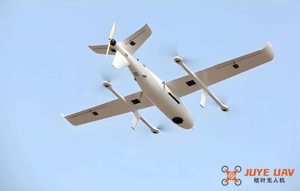
The figure above (inserted here as a conceptual illustration of a fixed-wing drone in flight) reminds us of the physical platform for which this control strategy was designed. While the image is not a simulation snapshot, it represents the typical small fixed-wing drone that benefits from the lightweight control logic.
| Waypoint | No Wind | Vertical 10 m/s | Headwind 10 m/s | Tailwind 10 m/s | Left Crosswind 5 m/s | Right Crosswind 5 m/s | Turbulence |
|---|---|---|---|---|---|---|---|
| 54-1 | 0 | 0 | 0 | 0 | 0 | 0 | 0 |
| 54-2 | 1116 | 1116 | 1146 | 973.4 | 1117 | 1117 | 1117 |
| 54-3 | 1252 | 1253 | 1284 | 1192 | 1251 | 1255 | 1252 |
| 53-1 (target) | 1598 | 1598 | 1605 | 1597 | 1598 | 1599 | 1598 |
Figure 2 (not shown here, but conceptually similar to the speed command plots mentioned in the original article) illustrates how the speed command adapts to different winds. For example, in headwind conditions, the commanded ground speed is higher to compensate for the wind drag, while in tailwind, it is lower. The drone’s indicated airspeed remains within the envelope, and the ground speed is adjusted accordingly.
The key observation is that the virtual drone model successfully guides the actual drone to the target within the required time window, even under significant wind disturbances. The strategy is computationally light because it primarily involves table lookups and a few algebraic operations each control cycle. This makes it highly suitable for small fixed-wing drones with limited processing power.
6. Conclusion
In this work, I have presented a timed arrival control strategy specifically tailored for small fixed-wing drones. By constructing a virtual drone ideal motion model that precomputes the desired time-velocity schedule along the route, and by continuously comparing the actual drone’s state with this model, the control system generates simple speed commands that achieve precise temporal and velocity constraints. The strategy accounts for wind disturbances through analytic formulas for ground speed and segment times, and it respects the drone’s performance envelope. Simulation results under various wind conditions demonstrate that the arrival time error is typically on the order of a few seconds, and the arrival speed matches the target. The computational efficiency of the approach makes it ideal for resource-constrained embedded systems commonly found in small fixed-wing drones. This capability enhances the autonomy of such drones, enabling them to participate in time-critical coordinated missions. Future work could extend the method to handle dynamic replanning in response to changing mission requirements or more complex wind fields.