
My fascination with the mesmerizing spectacle of a formation drone light show is not just about the beautiful patterns painted in the night sky. As a researcher in distributed control systems, I see it as a visible manifestation of profound technological challenges: precise coordination, robust communication, and, critically, the ability to dynamically adapt to an unpredictable environment. The true test of a formation’s intelligence lies not in its flawless geometric dance in open space, but in its graceful, cohesive evasion of unexpected obstacles while maintaining its artistic and functional intent. This article delves into the core control strategies that make such intelligent, obstacle-aware formation drone light shows and other multi-drone applications possible.
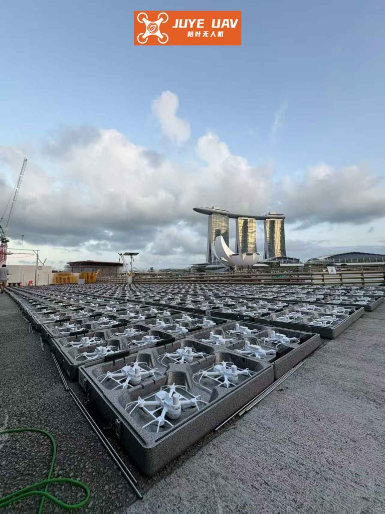
The pursuit of multi-drone systems is driven by their superior efficiency, redundancy, and capability over a single agent. Whether for search and rescue, agricultural monitoring, or an aerial formation drone light show, maintaining a specific spatial configuration is paramount. Among various strategies, the leader-follower approach within a distributed communication framework offers an excellent balance of simplicity, scalability, and robustness, making it highly suitable for real-world applications like a large-scale formation drone light show.
1. Mathematical Foundation of Formation Flight
To control a fleet, we must first model it. We consider a swarm of $n$ follower drones and one leader drone. Their communication network, defining who can talk to whom, is best described using graph theory. Let the directed graph $\mathcal{G} = (\Pi, \mathcal{E}, A_L)$ represent this network, where $\Pi = \{\pi_1, \pi_2, …, \pi_n\}$ is the set of follower nodes. The adjacency matrix $A_L = [a_{ij}] \in \mathbb{R}^{(n+1)\times(n+1)}$ encapsulates the links: $a_{ij}=1$ if drone $j$ can send information to drone $i$, and $a_{ii}=0$. The Laplacian matrix $L = D – A_L$, where $D$ is the diagonal in-degree matrix, along with a diagonal matrix $H$ indicating connection to the leader, defines the fundamental coupling structure for consensus-based control. The matrix $Q = L + H$ is crucial for stability analysis.
For control design, we often simplify the complex drone dynamics to a second-order point-mass model for the outer-loop position control, assuming a fast and well-tuned inner-loop attitude controller. The dynamics for drone $i$ are:
$$
\dot{\mathbf{r}}_i = \mathbf{v}_i, \quad \dot{\mathbf{v}}_i = \mathbf{u}_i
$$
where $\mathbf{r}_i = [x_i, y_i, z_i]^T$ and $\mathbf{v}_i$ are the position and velocity vectors, and $\mathbf{u}_i$ is the control input (acceleration). In state-space form, with $\mathbf{p}_i = [\mathbf{r}_i^T, \mathbf{v}_i^T]^T$, we have:
$$
\dot{\mathbf{p}}_i = A \mathbf{p}_i + B \mathbf{u}_i, \quad \text{with} \quad A = \begin{bmatrix} 0 & I_3 \\ 0 & 0 \end{bmatrix}, \quad B = \begin{bmatrix} 0 \\ I_3 \end{bmatrix}
$$
The collective dynamics for the entire formation of $n$ followers are:
$$
\dot{\mathbf{P}} = (I_n \otimes A) \mathbf{P} + (I_n \otimes B) \mathbf{U}
$$
where $\mathbf{P} = [\mathbf{p}_1^T, \mathbf{p}_2^T, …, \mathbf{p}_n^T]^T$, $\mathbf{U} = [\mathbf{u}_1^T, \mathbf{u}_2^T, …, \mathbf{u}_n^T]^T$, and $\otimes$ denotes the Kronecker product.
In the leader-follower paradigm, we define a desired offset $\mathbf{p}_i^* = [\mathbf{r}_i^{*T}, \mathbf{0}^T]^T$ for each follower relative to the leader’s state $\mathbf{p}_{n+1}$. The tracking error for follower $i$ is $\boldsymbol{\xi}_i = \mathbf{p}_i – \mathbf{p}_i^*$. The formation achieves its goal when all followers’ corrected states equal the leader’s state: $\boldsymbol{\xi}_1 = \boldsymbol{\xi}_2 = … = \boldsymbol{\xi}_n = \mathbf{p}_{n+1}$. We formalize the local consensus error for drone $i$ as:
$$
\mathbf{e}_i = \sum_{j=1}^{n} a_{ij}(\boldsymbol{\xi}_i – \boldsymbol{\xi}_j) + h_i (\boldsymbol{\xi}_i – \mathbf{p}_{n+1})
$$
A sliding surface is then constructed to drive this error to zero:
$$
\mathbf{s}_i = K \mathbf{e}_i, \quad \text{where} \quad K = [k_1 I_3, k_2 I_3], \: k_1, k_2 > 0
$$
The aggregated sliding surface vector for the formation is:
$$
\mathbf{S} = (Q \otimes K) \boldsymbol{\Xi} – (H \otimes K)(\mathbf{1}_n \otimes \mathbf{p}_{n+1})
$$
where $\boldsymbol{\Xi} = [\boldsymbol{\xi}_1^T, …, \boldsymbol{\xi}_n^T]^T$. Stability is guaranteed by ensuring the system trajectories reach and stay on $\mathbf{S} = \mathbf{0}$.
2. The Enhanced Artificial Potential Field
The classic Artificial Potential Field (APF) method provides a reactive, computationally light framework for obstacle avoidance, ideal for the real-time demands of a dynamic formation drone light show. However, it suffers from local minima and inefficient group behavior. Our enhanced APF addresses these flaws with four key components.
2.1 Repulsive Potential: Obstacles (modeled as spheres of radius $R_o$) generate a repulsive field within an influence radius $\rho_o$. The potential and force for obstacle $o$ on drone $i$ are:
$$
U_o(\mathbf{r}_i) =
\begin{cases}
\frac{1}{2} k_o \left( \frac{1}{d(\mathbf{r}_i, \mathbf{r}_o) – R_o} – \frac{1}{\rho_o} \right)^2, & \text{if } d \leq \rho_o \\
0, & \text{if } d > \rho_o
\end{cases}
$$
$$
\mathbf{F}_o(\mathbf{r}_i) = -\nabla U_o(\mathbf{r}_i) =
\begin{cases}
-k_o \left( \frac{1}{d – R_o} – \frac{1}{\rho_o} \right) \frac{\nabla d(\mathbf{r}_i, \mathbf{r}_o)}{(d – R_o)^2}, & \text{if } d \leq \rho_o \\
\mathbf{0}, & \text{if } d > \rho_o
\end{cases}
$$
where $d(\mathbf{r}_i, \mathbf{r}_o) = \|\mathbf{r}_i – \mathbf{r}_o\|$, $k_o>0$ is a gain, and $\nabla d(\mathbf{r}_i, \mathbf{r}_o)$ is the unit vector pointing from the obstacle to the drone. The total repulsive force is $\mathbf{F}_{o,\text{total}}(\mathbf{r}_i) = \sum_{o=1}^m \mathbf{F}_o(\mathbf{r}_i)$.
2.2 Attractive Potential: A traditional global attractive field can become too weak near obstacles. Our segmented design prevents this:
$$
U_{\text{att}}(\mathbf{r}_i) =
\begin{cases}
\frac{1}{2} k_{\text{att1}} d(\mathbf{r}_i, \mathbf{r}_t)^2, & \text{if } d(\mathbf{r}_i, \mathbf{r}_t) \leq d_{\text{thr}} \\
\frac{1}{2} k_{\text{att2}} d(\mathbf{r}_i, \mathbf{r}_t)^2, & \text{if } d(\mathbf{r}_i, \mathbf{r}_t) > d_{\text{thr}}
\end{cases}
$$
$$
\mathbf{F}_{\text{att}}(\mathbf{r}_i) = -\nabla U_{\text{att}}(\mathbf{r}_i) =
\begin{cases}
-k_{\text{att1}} (\mathbf{r}_i – \mathbf{r}_t), & \text{if } d \leq d_{\text{thr}} \\
-k_{\text{att2}} (\mathbf{r}_i – \mathbf{r}_t), & \text{if } d > d_{\text{thr}}
\end{cases}
$$
with $k_{\text{att1}} > k_{\text{att2}} > 0$. This ensures a stronger pull when the drone is closer to the target $\mathbf{r}_t$, enhancing goal convergence in cluttered spaces.
2.3 Formation Coordination Potential: This is the cornerstone for efficient formation drone light show obstacle avoidance. Instead of dissolving the formation, this field temporarily deforms it. It activates only for drones under repulsive influence (flag$_i=1$). It uses the communication graph $A_L$ to calculate a force that pulls a drone towards its *correct relative position* within the moving formation, counteracting disruptive repulsive forces:
$$
U_b(\mathbf{r}_i, \{\mathbf{r}_j\}) =
\begin{cases}
\frac{k_b}{\sum_{j \neq i} a_{ij}} \sum_{j \neq i}^{n+1} a_{ij} \left[ d(\mathbf{r}_i, \mathbf{r}_j) + \frac{\|\mathbf{p}_i^* – \mathbf{p}_j^*\|^2}{d(\mathbf{r}_i, \mathbf{r}_j)} \right], & \text{if flag}_i=1 \\
0, & \text{if flag}_i=0
\end{cases}
$$
The resulting coordination force is:
$$
\mathbf{F}_b(\mathbf{r}_i, \{\mathbf{r}_j\}) =
\begin{cases}
-\frac{k_b}{\sum_{j \neq i} a_{ij}} \sum_{j \neq i}^{n+1} a_{ij} \left[ 1 – \frac{\|\mathbf{p}_i^* – \mathbf{p}_j^*\|^2}{d(\mathbf{r}_i, \mathbf{r}_j)^2} \right] \nabla d(\mathbf{r}_i, \mathbf{r}_j), & \text{if flag}_i=1 \\
\mathbf{0}, & \text{if flag}_i=0
\end{cases}
$$
This term minimizes formation distortion and also provides inter-drone collision avoidance.
2.4 Auxiliary Escape Potential: To solve the local minima problem, this tangential field activates when a drone’s movement over recent timesteps falls below a threshold $\delta$, indicating stagnation. It provides a “nudge” perpendicular to the repulsive force gradient to escape the trap:
$$
U_h(\mathbf{r}_i) =
\begin{cases}
\frac{1}{2} k_h d(\mathbf{r}_i, \mathbf{r}_o)^2, & \text{if } \Delta d_i \leq \delta \\
0, & \text{otherwise}
\end{cases}
$$
$$
\mathbf{F}_h(\mathbf{r}_i) = -\nabla U_h(\mathbf{r}_i) =
\begin{cases}
-k_h (\mathbf{r}_i – \mathbf{r}_o), & \text{if } \Delta d_i \leq \delta \\
\mathbf{0}, & \text{otherwise}
\end{cases}
$$
The total improved potential field force on a follower drone is:
$$
\mathbf{F}_{\text{total}}(\mathbf{r}_i) = \mathbf{F}_{\text{att}}(\mathbf{r}_i) + \mathbf{F}_{o,\text{total}}(\mathbf{r}_i) + \mathbf{F}_{b}(\mathbf{r}_i, \{\mathbf{r}_j\}) + \mathbf{F}_{h}(\mathbf{r}_i)
$$
3. Distributed Sliding Mode Formation Controller with Integrated Obstacle Avoidance
Our control architecture seamlessly integrates the enhanced APF into the sliding mode formation controller, enabling true cooperative obstacle avoidance rather than a simple dissolve-and-reform strategy.
3.1 Leader Trajectory Control: The leader’s motion is governed by the improved APF, guiding the entire formation.
$$
\mathbf{u}_{n+1}(t) = \mathbf{F}_{\text{att}}(\mathbf{r}_{n+1}) + \mathbf{F}_{o,\text{total}}(\mathbf{r}_{n+1}) + \mathbf{F}_{h}(\mathbf{r}_{n+1}) – k_L \dot{\mathbf{r}}_{n+1}
$$
The damping term $-k_L \dot{\mathbf{r}}_{n+1}$ ensures control input boundedness.
3.2 Follower Distributed Cooperative Controller: This is the core innovation. When a follower encounters an obstacle, the APF force $\mathbf{F}_{\text{total}}(\mathbf{r}_i)$ is not treated as a separate, overriding command. Instead, it is used to temporarily modify the follower’s desired formation offset:
$$
\tilde{\mathbf{p}}_i^*(t) = \mathbf{p}_i^* + [\mathbf{F}_{\text{total}}(\mathbf{r}_i)^T, \mathbf{0}^T]^T
$$
This adjusted reference $\tilde{\mathbf{P}}^*(t)$ is then fed into the sliding mode formation controller. The control law $\mathbf{U}(t) = \mathbf{U}_{eq}(t) + \mathbf{U}_{sw}(t)$ is derived to drive $\mathbf{S}$ to zero.
The equivalent control $\mathbf{U}_{eq}$ is designed based on the nominal dynamics:
$$
\mathbf{U}_{eq}(t) = – (Q \otimes KB)^{-1} \left\{ [Q \otimes KA] \mathbf{P} – (Q \otimes K) \dot{\tilde{\mathbf{P}}}^* – H \mathbf{1}_n \otimes (K A \mathbf{p}_{n+1} + K B \boldsymbol{\sigma}) \right\}
$$
where $\boldsymbol{\sigma}$ is a lower bound for the leader’s control input.
The switching control $\mathbf{U}_{sw}$ ensures robustness and finite-time convergence, using a hyperbolic tangent function to reduce chattering:
$$
\mathbf{U}_{sw}(t) = – (Q \otimes KB)^{-1} \left[ \lambda_1 \tanh(\mathbf{S}) + \lambda_2 \mathbf{S} \right], \quad \lambda_1, \lambda_2 > 0
$$
The final distributed sliding mode cooperative obstacle avoidance control protocol is:
$$
\begin{aligned}
\mathbf{U}(t) = & – (Q \otimes KB)^{-1} \bigl( [Q \otimes KA] \mathbf{P} – (Q \otimes K) \dot{\tilde{\mathbf{P}}}^* \\
& – H \mathbf{1}_n \otimes (K A \mathbf{p}_{n+1} + K B \boldsymbol{\sigma}) + \lambda_1 \tanh(\mathbf{S}) + \lambda_2 \mathbf{S} \bigr)
\end{aligned}
$$
This controller ensures that followers simultaneously track the dynamically adjusted formation setpoints (which encode obstacle avoidance commands) and maintain consensus with their neighbors. The formation fluidly deforms around obstacles and rapidly reconstructs afterward, minimizing the performance degradation seen in dissolution-based methods. This is essential for a continuous and spectacular formation drone light show over complex terrain.
4. Performance Analysis and Comparative Results
The stability of the closed-loop system under the proposed controller can be rigorously proven using Lyapunov theory, showing that the sliding surface $\mathbf{S}$ is reached in finite time and the formation errors converge.
To quantify the advantage of our cooperative deformation strategy over the traditional dissolve-and-reform strategy, we can analyze key metrics through simulation. The following table summarizes a conceptual comparison:
| Performance Metric | Dissolve-and-Reform Strategy | Proposed Cooperative Deformation Strategy |
|---|---|---|
| Formation Integrity During Avoidance | Low (Formation dissolves) | High (Formation deforms cohesively) |
| Inter-Agent Coordination | Minimal (Individual obstacle avoidance) | High (Coordinated motion via $\mathbf{F}_b$) |
| Post-Avoidance Re-formation Time | Slow | Fast |
| Efficiency of Path (Total Distance) | Longer (Erratic individual paths) | Shorter (Smooth, group-optimized path) |
| Suitability for Formation Drone Light Show | Poor (Causes visible breaks in show) | Excellent (Maintains visual continuity) |
A critical metric is the Formation Loss Coefficient $C$, which measures the spatial dispersion of the swarm relative to its centroid:
$$
C = \frac{1}{n+1} \sum_{i=1}^{n+1} \| \mathbf{r}_i – \bar{\mathbf{r}} \|, \quad \text{where} \quad \bar{\mathbf{r}} = \frac{1}{n+1} \sum_{i=1}^{n+1} \mathbf{r}_i
$$
In simulations, a formation using our controller will exhibit smaller and shorter-duration peaks in $C$ when encountering obstacles compared to a dissolve-and-reform controller. This quantitatively proves our method’s superior ability to preserve formation integrity, a non-negotiable requirement for a flawless formation drone light show or a precise military or industrial inspection fleet.
5. Conclusion and Future Directions
The integration of an improved artificial potential field with a distributed sliding mode control framework presents a powerful solution for multi-drone cooperative obstacle avoidance. By addressing the key shortcomings of traditional APF—local minima and poor group behavior—and embedding the avoidance directives directly into the formation tracking errors, we enable a swarm to navigate cluttered environments with minimal degradation to its formation quality. This approach ensures rapid obstacle negotiation and swift re-formation, which is vital for mission efficiency and, in the case of a formation drone light show, for maintaining an uninterrupted and captivating aerial performance.
The future of this field lies in extending these principles to fully dynamic environments with moving obstacles and other drones, incorporating more sophisticated communication protocols with delays and dropouts, and adapting the algorithms for highly nonlinear drone dynamics. As the technology matures, the complexity and reliability of large-scale, intelligent formation drone light shows will only increase, pushing the boundaries of what is possible in coordinated aerial systems.