
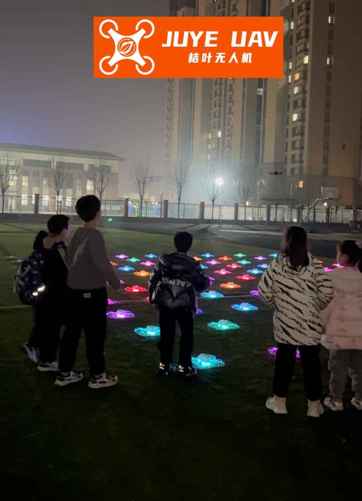
The spectacle of a formation drone light show is a mesmerizing fusion of art and technology. Hundreds, sometimes thousands, of unmanned aerial vehicles (UAVs) move in perfect harmony across the night sky, creating intricate, dynamic three-dimensional shapes and animations. This capability offers advantages unattainable by a single drone, transforming entertainment, advertising, and large-scale ceremonies. However, the breathtaking precision of these aerial ballets hinges on a critical technological foundation: accurate, real-time knowledge of each drone’s state relative to its neighbors and the intended formation pattern. Any uncertainty in this knowledge—due to unpredictable wind gusts, sensor noise, or modeling inaccuracies—can cascade into visible desynchronization, ruining the illusion and posing safety risks. This article explores a robust estimation framework, born from advanced control theory, that is pivotal for achieving the resilience and accuracy required for next-generation formation drone light show systems.
At its core, a drone in a formation drone light show must solve a navigation and control problem. It needs to know precisely where it is, where its neighboring drones are, and where it needs to go next in the choreography. While Global Navigation Satellite Systems (GNSS) like GPS provide absolute positioning, they are susceptible to errors, multipath effects (especially in urban canyons where shows are often held), and, in extreme cases, jamming. Relying solely on GNSS makes the formation vulnerable. Therefore, augmenting absolute positioning with relative sensing between drones is crucial for maintaining tight formation geometry. Vision-based systems, using onboard cameras, offer a compelling solution for relative navigation as they are passive, low-cost, and do not require external infrastructure. However, they introduce their own set of challenges, primarily the inherent uncertainty when estimating the complete three-dimensional state of neighboring drones from two-dimensional image data, particularly the challenging-to-estimate relative range.
The visual estimation challenge is exacerbated when drones execute aggressive maneuvers as part of the show’s choreography. A key unknown in the state estimation problem becomes the acceleration of the neighboring or “leader” drone in the formation pair. If this maneuver is not properly accounted for, the estimating (“follower”) drone’s understanding of the leader’s future position degrades rapidly, leading to lag and error in its own tracking control. This is fundamentally a problem of state estimation for a system with significant uncertainties and unmodeled dynamics. The classical tool for state estimation is the Kalman filter, but its performance can severely deteriorate if target maneuver uncertainties are not compensated. This article delves into a sophisticated estimation strategy that combines the predictive power of a time-varying Kalman filter with the adaptive, learning capability of neural networks to tackle precisely this problem, ensuring the robustness of the formation drone light show.
The State Estimation Problem in Drone Formations
We begin by formalizing the estimation problem for a general multi-input, multi-output (MIMO) uncertain system, which perfectly encapsulates the dynamics between two drones in a formation. Consider the following system representation, where the state of a neighboring drone (or a virtual reference point in the formation) must be estimated:
$$ \dot{x} = A x + B u + f(x, t) $$
$$ y = C x + D v(t) $$
Here, \( x \in \mathbb{R}^n \) represents the true state vector to be estimated. This state typically includes relative position, velocity, and potentially acceleration components between drones in the formation drone light show. The term \( A x + B u \) describes the nominal, known dynamics of the system. The critical component is \( f(x, t) \), which represents the lumped uncertainty. This function encapsulates all unknown or difficult-to-model effects, such as:
- Unpredictable aerodynamic disturbances (wind gusts).
- Unmodeled actuator dynamics or delays.
- The unknown acceleration component of a maneuvering neighbor drone in the formation.
- Nonlinearities in the vision-based measurement process.
The function \( f(x, t) \) is assumed to be bounded but otherwise unknown. The output \( y \in \mathbb{R}^m \) is the measurement available to the drone, for instance, the line-of-sight (LOS) angles (azimuth and elevation) derived from its camera, combined with perhaps a noisy relative range estimate from another sensor. The matrix \( C \) is the output matrix, and \( D v(t) \) represents measurement noise.
The core objective is to design an estimation algorithm that produces an estimate \( \hat{x} \) of the true state \( x \), such that the estimation error \( e = x – \hat{x} \) remains bounded and as small as possible, even in the persistent presence of the unknown nonlinearity \( f(x, t) \). This is the bedrock of reliable autonomy for a formation drone light show.
For the specific case of a vision-based formation drone light show, the states and measurements can be detailed. Let us define the relative states between a follower drone and its leader (or formation reference) in a 3D inertial frame. The key parameters are the relative range \( r \), the azimuth angle \( \lambda_a \), and the elevation angle \( \lambda_e \).
| Symbol | Description |
|---|---|
| \( r \) | Relative distance between drones. |
| \( \lambda_a \) | Azimuth angle (bearing) to the neighbor drone. |
| \( \lambda_e \) | Elevation angle to the neighbor drone. |
| \( \dot{r} \) | Line-of-sight (LOS) range rate. |
| \( \dot{\lambda}_a, \dot{\lambda}_e \) | LOS angular rates. |
| \( a_{Lx}, a_{Ly}, a_{Lz} \) | Unknown accelerations of the neighbor/leader drone. |
The dynamics of these LOS parameters can be derived from relative kinematics. The state vector for estimation can be chosen as \( x = [r, \lambda_a, \lambda_e, \dot{r}, \dot{\lambda}_a, \dot{\lambda}_e]^T \) or a higher-order one including relative positions and velocities. The nonlinear function \( f(x, t) \) prominently contains the projections of the leader’s unknown acceleration \( (a_{Lx}, a_{Ly}, a_{Lz}) \) onto the LOS coordinates. The measurement \( y \) might be the directly measurable angles and a rough range estimate:
$$ y = [\lambda_a + \nu_a, \lambda_e + \nu_e, r + \nu_r]^T $$
where \( \nu \) terms represent measurement noise. The challenge is to estimate the full state \( x \), especially the velocities and the hidden acceleration effects, from these limited and noisy measurements.
Robust Time-Varying Kalman Filter with Neural Network Augmentation
To address the estimation problem with uncertainties, we propose a Robust Time-Varying Kalman Filter (RTVKF) augmented with an Adaptive Neural Network (ANN). This hybrid structure leverages the optimality of the Kalman filter for linear Gaussian systems while using the ANN’s universal approximation capability to learn and cancel the nonlinear uncertainty \( f(x, t) \) online. This is crucial for a formation drone light show operating in changing environmental conditions.
The standard Kalman filter provides an estimate \( \hat{x}_{kf} \) based on the nominal model:
$$ \dot{\hat{x}}_{kf} = A \hat{x}_{kf} + B u + K(t) (y – C \hat{x}_{kf}) $$
The time-varying Kalman gain \( K(t) \) is computed from:
$$ K(t) = P(t) C^T R^{-1} $$
where \( P(t) \) is the solution to the differential Riccati equation:
$$ \dot{P}(t) = A P(t) + P(t) A^T + Q – P(t) C^T R^{-1} C P(t) $$
with \( Q \) and \( R \) being the process and measurement noise covariance matrices, respectively. However, this filter’s error dynamics are corrupted by the unknown \( f(x, t) \):
$$ \dot{e}_{kf} = (A – K(t)C) e_{kf} + f(x, t) – K(t)D v(t) $$
Clearly, \( f(x, t) \) acts as a persistent disturbance, causing bias and potentially unbounded error.
The proposed solution is to augment the filter with a direct estimate of the uncertainty. We approximate \( f(x, t) \) using a Radial Basis Function (RBF) neural network:
$$ f(x, t) = W^{*T} \Phi(x, t) + \epsilon(x, t) $$
Here, \( W^* \) is the ideal (unknown) weight matrix, \( \Phi(x, t) \) is the vector of basis functions (e.g., Gaussian functions), and \( \epsilon \) is the bounded approximation error. Since \( W^* \) is unknown, we maintain an online estimate \( \hat{W} \). The robust estimator is then formulated as:
$$ \dot{\hat{x}} = A \hat{x} + B u + \hat{W}^T \Phi(\hat{x}, t) + K(t) (y – C \hat{x}) $$
The key innovation lies in the training of the neural network weights \( \hat{W} \). Instead of using just the output error \( (y – C\hat{x}) \), which is filtered through \( K(t) \), we define a composite error signal for stronger learning. Let \( e = x – \hat{x} \). We construct a training signal that combines the output estimation error and a filtered state prediction error, leading to faster and more stable convergence of the neural network weights.
The weight update law for the \( i \)-th network weight vector \( \hat{w}_i \) is designed using a gradient-based adaptive rule:
$$ \dot{\hat{w}}_i = -\Gamma_i \left[ \Phi(\hat{x}, t) s_i + \kappa_i \hat{w}_i \right] $$
where:
- \( s_i \) is the \( i \)-th component of the carefully designed composite error vector \( s \).
- \( \Gamma_i \) is a positive definite learning rate matrix.
- \( \kappa_i \) is a small positive scalar for leakage (sigma-modification), which ensures boundedness of weights without requiring persistent excitation, a critical feature for a formation drone light show where maneuvers may not always excite all dynamics.
This update law drives the neural network to learn the uncertainty \( f(x, t) \) online. As \( \hat{W} \) converges towards \( W^* \), the term \( \hat{W}^T \Phi(\hat{x}, t) \) cancels out \( f(x, t) \) in the error dynamics, leaving a system dominated by the stable dynamics of \( (A – K(t)C) \).
| Method | Principle | Advantages | Disadvantages for Light Shows |
|---|---|---|---|
| Standard EKF | Linearizes nonlinear model. | Computationally efficient, widely used. | Performance degrades with large model uncertainty and unmodeled leader maneuvers. |
| Multiple Model Adaptive Estimation (MMAE) | Runs multiple filters for different maneuver models. | Can handle discrete maneuver changes. | Computationally heavy; model set may not cover all continuous show choreography. |
| Interactive Multiple Model (IMM) | Blends estimates from multiple model-matched filters. | More robust than MMAE. | Still model-dependent; tuning complexity is high. |
| Proposed RTVKF+ANN | Uses ANN to directly learn and compensate uncertainties. | Model-independent, highly robust to continuous unknown inputs (maneuvers/wind), adaptive. | Requires careful tuning of ANN parameters; slightly higher computational load than EKF. |
Boundedness and Stability Analysis
For any algorithm intended for a safety-critical application like a formation drone light show, a formal proof of stability and boundedness is non-negotiable. We analyze the error dynamics of the overall system, comprising the state estimation error \( e = x – \hat{x} \) and the neural network weight estimation error \( \tilde{W} = W^* – \hat{W} \).
Using the system dynamics and the robust estimator equation, the state error dynamics can be derived as:
$$ \dot{e} = (A – K(t)C) e + \tilde{W}^T \Phi(\hat{x}, t) + \epsilon(x, t) – K(t)D v(t) $$
The weight error dynamics come from the update law:
$$ \dot{\tilde{W}} = -\dot{\hat{W}} = \Gamma \Phi(\hat{x}, t) s^T + \kappa \Gamma \hat{W} $$
The composite error \( s \) is typically a function of \( e \) (e.g., \( s = e + \alpha \int e \, dt \)).
To prove boundedness, we construct a Lyapunov function candidate, a positive definite function that measures the overall “energy” of the errors. A standard choice is:
$$ V = \frac{1}{2} e^T P^{-1} e + \frac{1}{2} \text{tr}(\tilde{W}^T \Gamma^{-1} \tilde{W}) $$
where \( P(t) \) is the solution to the Riccati equation and is bounded and positive definite. Taking the time derivative of \( V \) along the trajectories of the error system and substituting the dynamics yields:
$$ \dot{V} \leq -\frac{1}{2} e^T (P^{-1}Q_m P^{-1}) e + e^T P^{-1} (\epsilon – K D v) + \text{tr}(\tilde{W}^T \Phi s^T) – \kappa \text{tr}(\tilde{W}^T \hat{W}) + \text{…} $$
Here, \( Q_m \) is a positive definite matrix related to the Riccati equation. By employing Young’s inequality and the boundedness properties of \( \epsilon \), \( v \), and the basis functions \( \Phi \), we can manipulate this expression into the form:
$$ \dot{V} \leq -\alpha V + \beta $$
where \( \alpha \) and \( \beta \) are positive constants. This inequality is the key. It shows that when the error “energy” \( V \) is large, the term \( -\alpha V \) dominates, pulling \( V \) down. It can only grow until \( \dot{V} \) becomes zero, which happens when \( V \leq \beta / \alpha \). This is a classic result in stability theory, proving that \( V \), and consequently the errors \( e \) and \( \tilde{W} \), are uniformly ultimately bounded (UUB). All signals in the closed-loop estimation system remain within a compact set. The size of the ultimate bound can be made smaller by increasing the learning gains \( \Gamma \) (to reduce approximation error impact) and the filter gains (via \( Q \), \( R \)), but practical constraints like measurement noise and computational limits must be respected. This boundedness guarantee is essential for ensuring that the state estimate for a drone in a formation drone light show never diverges catastrophically, even during aggressive, unmodeled show maneuvers.
Application to Formation Flight Control in Light Shows
How does this robust estimator integrate into the complete control stack of a formation drone light show? The estimated states are not an end in themselves; they are the critical inputs to the formation-keeping and trajectory-tracking controllers on each drone.
The overall architecture for a follower drone in a decentralized formation drone light show can be summarized in the following steps, which form a continuous loop:
- Sensor Fusion: Raw measurements from GNSS, IMU, and vision/lidar sensors are pre-processed.
- Robust Relative State Estimation (RTVKF+ANN): This module, detailed in this article, takes the processed measurements (like LOS angles \(y\)) and produces a robust estimate \( \hat{x} \) of the relative state (position, velocity) of key neighbor drones or the formation’s virtual reference structure. It actively learns and compensates for unknown disturbances and neighbor accelerations.
- Formation Control Law: The estimated relative state \( \hat{x} \) is fed into a control algorithm (e.g., a nonlinear dynamic inversion controller, a robust sliding mode controller, or a model predictive controller). This controller computes the required forces and moments. For a typical quadrotor drone in a formation drone light show, this translates into desired thrust and attitude commands.
- Low-Level Attitude Control: The desired attitude is tracked by a fast, inner-loop attitude controller, which commands motor speeds.
- Actuation: Electronic speed controllers (ESCs) drive the motors to achieve the commanded speeds, ultimately producing the physical motion that closes the loop.
The value of the RTVKF+ANN estimator is most apparent in steps 2 and 3. Consider a show segment where drones are instructed to perform a rapid “flower blooming” maneuver, involving simultaneous outward radial acceleration. A standard Kalman filter, assuming constant velocity, would persistently underestimate the relative velocity and position of neighbors leading to a laggy, sluggish response from the follower drones. In contrast, the ANN in the RTVKF+ANN architecture quickly learns the pattern of this radial acceleration from the composite error signal. It injects a compensating term \( \hat{W}^T \Phi \) into the state estimate, allowing the filter’s internal model to effectively “predict” the neighbor’s motion more accurately. This results in a more accurate \( \hat{x} \) being sent to the formation controller, enabling the follower drone to command the correct thrust and attitude proactively, maintaining the precise geometric shape of the “blooming flower” throughout the dynamic maneuver.
The performance of this integrated system can be quantified. The primary metrics for a formation drone light show are:
- Formation Tracking Error: The RMS error in relative position between drones compared to the desired choreography.
- Maximum Collision Risk Probability: Derived from the covariance estimates \( P(t) \) of the filter, indicating uncertainty ellipsoids.
- Control Effort (Energy Consumption): Integrated thrust usage over the show duration.
A well-tuned RTVKF+ANN estimator directly minimizes the tracking error and the covariance bounds, leading to a safer, more precise, and potentially more energy-efficient show, as the drones don’t waste energy on corrective maneuvers due to poor estimates.
Conclusion and Future Perspectives
The pursuit of ever more spectacular and reliable formation drone light show demands continuous advancement in core technologies, with state estimation being a cornerstone. The Robust Time-Varying Kalman Filter augmented with an Adaptive Neural Network presents a powerful solution to the problem of estimating drone states amid significant uncertainties like unknown neighbor maneuvers and environmental disturbances. By formally guaranteeing bounded estimation errors and leveraging the universal approximation power of neural networks, this approach provides the resilience needed for large-scale, outdoor, dynamic drone choreographies.
Looking forward, several exciting research avenues can build upon this foundation to further revolutionize formation drone light show technology:
| Direction | Description | Potential Impact |
|---|---|---|
| Distributed & Collaborative Estimation | Drones share local estimates or features (not raw data) to collaboratively build a consistent global picture of the formation’s state, enhancing robustness to individual sensor failure. | Enables truly scalable shows with thousands of drones, maintaining coherence even if some drones lose GPS. |
| Deep Learning for Uncertainty Modeling | Using deep neural networks or recurrent networks (LSTMs) instead of RBF networks to learn more complex, temporal patterns in disturbances and complex aerodynamic interactions between closely-flying drones (downwash effects). | Could handle even more extreme and unpredictable show choreographies and weather conditions. |
| Integration with Event- or Feature-Based Vision | Coupling the estimator with advanced vision sensors like event cameras, which are exceptionally good at tracking fast motion, or direct feature trackers that bypass explicit state-space models. | Would drastically improve performance during the fastest, most dazzling segments of a light show. |
| Formal Synthesis for Safety Guarantees | Using techniques from robust control and formal methods to synthesize the estimator and controller together, providing mathematically proven safe operating envelopes (e.g., guaranteed minimum separation). | Critical for regulatory approval and safe operation over crowds in dense urban environments. |
The fusion of rigorous control theory with adaptive learning algorithms, as exemplified by the RTVKF+ANN, is key to unlocking the full artistic and technical potential of formation drone light show. As these technologies mature, we can anticipate not just more complex shapes, but emotionally intelligent, real-time interactive displays that respond to music, audience movement, or environmental factors, all while operating with the unwavering precision and safety that modern audiences and regulators will demand. The sky is not the limit; it is the canvas, and robust estimation is the brush that allows us to paint upon it with light and motion.