
In recent years, formation drone light shows have captivated audiences worldwide, where multiple unmanned aerial vehicles (UAVs) coordinate to create dazzling aerial displays. As a researcher in autonomous systems, I have explored advanced control strategies to enhance the precision and reliability of these performances. This paper presents my work on designing a sliding mode controller for formation drone light shows, focusing on maintaining and transforming intricate patterns in three-dimensional space. The core challenge lies in ensuring that drones can swiftly adapt to dynamic commands while avoiding collisions, a task that demands robust control algorithms. Here, I leverage sliding mode variable structure control due to its inherent robustness against disturbances and model uncertainties, which are common in outdoor environments where formation drone light shows are staged.
Formation drone light shows involve fleets of UAVs operating in close proximity to form geometric shapes or moving patterns. Traditional control methods, such as PID, often struggle with rapid maneuvers and external interferences like wind gusts. My approach builds upon existing research in UAV formation flight but tailors it specifically for entertainment applications. The key innovation is the decomposition of the control problem into lateral, longitudinal, and vertical channels, each governed by a dedicated sliding mode controller. This modular design simplifies tuning and improves response times, crucial for synchronized movements in formation drone light shows. Throughout this article, I will detail the mathematical modeling, controller design, and simulation results, emphasizing how this method outperforms conventional techniques in maintaining and transforming formations.
The foundation of any formation drone light show control system is a accurate mathematical model that captures the kinematics and dynamics of the drones. I consider a scenario where multiple drones, referred to as leaders and followers, must maintain specific relative positions. Inspired by conventional autopilot models, I represent each drone’s motion using first-order speed hold, second-order heading hold, and second-order altitude hold dynamics. For a follower drone relative to a leader in a formation drone light show, the state-space equations are derived from geometric relationships in 3D space. Let me define the inertial coordinate system and the follower’s rotating reference frame, where the x-axis aligns with the follower’s instantaneous velocity. The relative position errors in lateral (y), longitudinal (x), and vertical (z) directions form the basis for control.
The dynamics of a follower drone in a formation drone light show can be expressed as follows, where subscript \(i\) denotes the drone (leader \(L\) or follower \(W\)):
$$ \tau_V \dot{V}_i = -V_i + V_{ic} $$
$$ \tau_{\psi a} \tau_{\psi b} \ddot{\psi}_i = -(\tau_{\psi a} + \tau_{\psi b}) \dot{\psi}_i – \psi_i + \psi_{ic} $$
$$ \tau_{ha} \tau_{hb} \ddot{h}_i = -(\tau_{ha} + \tau_{hb}) \dot{h}_i – h_i + h_{ic} $$
Here, \(V\) is velocity, \(\psi\) is heading angle, \(h\) is altitude, and \(\tau\) parameters are time constants. For formation control, I define the relative states: \(x\) (longitudinal distance), \(y\) (lateral distance), and \(z = h_W – h_L\) (vertical distance). The kinematic equations coupling these states are:
$$ \dot{x} = V_L \cos(\psi_L – \psi_W) – V_W + y \dot{\psi}_W $$
$$ \dot{y} = V_L \sin(\psi_L – \psi_W) – x \dot{\psi}_W $$
$$ \dot{z} = \dot{h}_W – \dot{h}_L $$
Combining these with the autopilot models yields a full state-space representation for the formation drone light show system. I denote the state vector as \(\mathbf{X} = [x, V_W, y, \psi_W, \dot{\psi}_W, z, \dot{z}]^T\), with control inputs \(V_{Wc}\), \(\psi_{Wc}\), and \(h_{Wc}\) for the follower, and leader states as disturbances. This model is decoupled into three channels for controller design, as summarized in Table 1.
| Channel | States | Control Input | Primary Objective |
|---|---|---|---|
| Longitudinal (X) | \(x, V_W\) | \(V_{Wc}\) | Maintain desired front-back spacing |
| Lateral (Y) | \(y, \psi_W, \dot{\psi}_W\) | \(\psi_{Wc}\) | Maintain desired side spacing and heading alignment |
| Vertical (Z) | \(z, \dot{z}\) | \(h_{Wc}\) | Maintain desired altitude difference |
This decoupling simplifies the controller design for formation drone light shows, allowing me to address each spatial dimension independently. The lateral and vertical channels are fully decoupled, while the longitudinal channel couples with lateral through heading rate terms, which I handle via feedback linearization. Next, I will delve into the sliding mode controller design for each channel, a cornerstone of my approach to achieving robust performance in formation drone light shows.
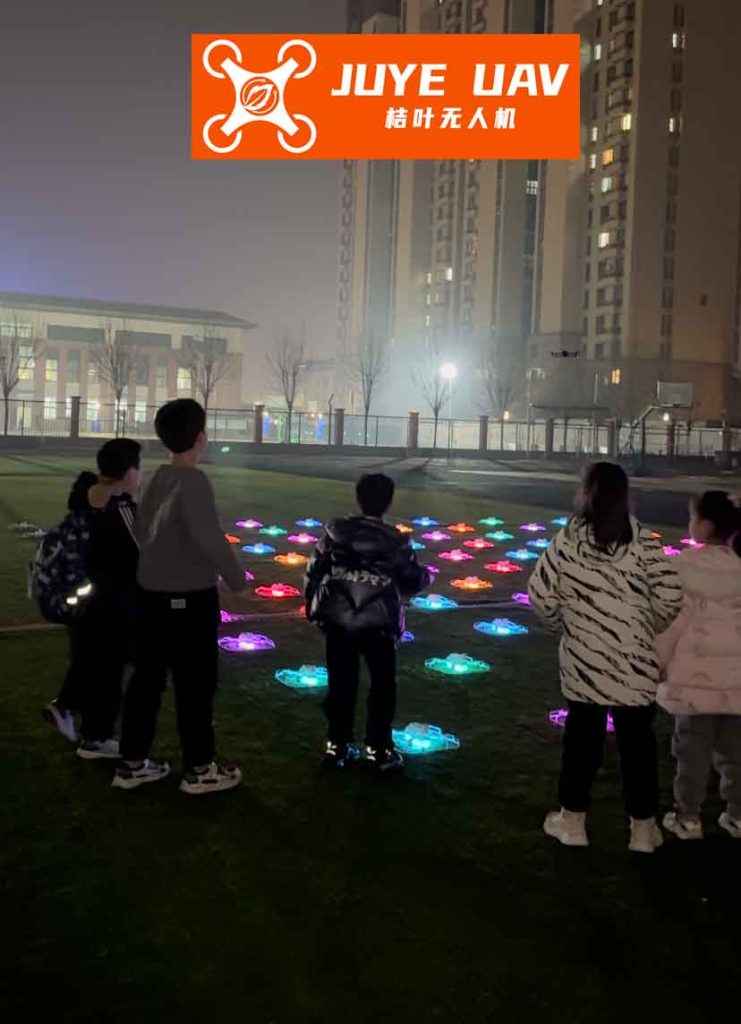
Sliding mode control is renowned for its invariance to matched uncertainties, making it ideal for formation drone light shows where environmental disturbances are unpredictable. My design employs different reaching laws for each channel to balance convergence speed and chattering reduction. For the lateral (Y) channel, I use an exponential reaching law; for the vertical (Z) channel, a constant rate reaching law; and for the longitudinal (X) channel, an exponential reaching law with feedback linearization. Let me outline the design process for each, incorporating key formulas that ensure stability and precision in formation drone light shows.
Starting with the lateral channel, which controls the side spacing \(y\) and heading synchronization, the state equations are:
$$ \dot{y} = V_L \sin(\psi_L – \psi_W) – x \dot{\psi}_W $$
$$ \ddot{y} = f_y(\mathbf{x}) – \frac{1}{\tau_{\psi a} \tau_{\psi b}} \cos(\alpha) \psi_{Wc} $$
where \(\alpha\) is the formation angle, and \(f_y(\mathbf{x})\) aggregates other terms. Defining the tracking error \(e_y = y – y_d\) for desired spacing \(y_d\), I choose the sliding surface \(s_y = \dot{e}_y + k_{1y} e_y\) with \(k_{1y} > 0\). Using the exponential reaching law \(\dot{s}_y = -\epsilon_y \text{sgn}(s_y) – k_{2y} s_y\), where \(\epsilon_y, k_{2y} > 0\), the control law for heading command becomes:
$$ \psi_{Wc} = \frac{\tau_{\psi a} \tau_{\psi b}}{\cos(\alpha)} \left( f_y(\mathbf{x}) + \ddot{y}_d – k_{1y} \dot{e}_y + \epsilon_y \text{sgn}(s_y) + k_{2y} s_y \right) $$
This ensures that \(s_y \dot{s}_y < 0\), driving the system to the sliding manifold where \(e_y \to 0\). For formation drone light shows, this guarantees accurate lateral positioning even during sharp turns.
For the vertical channel, which manages altitude differences, the dynamics are simpler. Let \(e_z = z – z_d\) and choose sliding surface \(s_z = \dot{e}_z + c_z e_z\) with \(c_z > 0\). Applying a constant rate reaching law \(\dot{s}_z = -\eta_z \text{sgn}(s_z)\), the altitude control input is:
$$ h_{Wc} = \tau_{ha} \tau_{hb} \left( \frac{1}{\tau_{ha} \tau_{hb}} \dot{h}_W + \ddot{h}_L – c_z \dot{e}_z + \eta_z \text{sgn}(s_z) \right) $$
This provides robust height tracking, essential for maintaining layered patterns in formation drone light shows, such as cascading waves or spirals.
The longitudinal channel controls forward spacing \(x\) and velocity matching. After feedback linearization to decouple terms, I define error \(e_x = x – x_d\) and sliding surface \(s_x = \dot{e}_x + k_{1x} e_x\). Using an exponential reaching law, the velocity command is:
$$ V_{Wc} = \tau_V \left( f_x(\mathbf{x}) + \ddot{x}_d – k_{1x} \dot{e}_x + \epsilon_x \text{sgn}(s_x) + k_{2x} s_x \right) $$
where \(f_x(\mathbf{x})\) includes coupling effects. This ensures fast convergence for spacing adjustments, critical when transitioning between shapes in a formation drone light show. The parameters for each channel are tuned via simulation, as detailed later. To summarize the controller structure, I present Table 2, which links each channel’s components to the overall goals of formation drone light shows.
| Channel | Sliding Surface | Reaching Law | Key Parameters | Role in Formation Drone Light Show |
|---|---|---|---|---|
| Lateral (Y) | \(s_y = \dot{e}_y + k_{1y} e_y\) | Exponential: \(\dot{s}_y = -\epsilon_y \text{sgn}(s_y) – k_{2y} s_y\) | \(k_{1y}=10, k_{2y}=10, \epsilon_y=0.5\) | Ensures side spacing accuracy for symmetric patterns |
| Vertical (Z) | \(s_z = \dot{e}_z + c_z e_z\) | Constant: \(\dot{s}_z = -\eta_z \text{sgn}(s_z)\) | \(c_z=1, \eta_z=0.3\) | Maintains altitude layers for 3D effects |
| Longitudinal (X) | \(s_x = \dot{e}_x + k_{1x} e_x\) | Exponential: \(\dot{s}_x = -\epsilon_x \text{sgn}(s_x) – k_{2x} s_x\) | \(k_{1x}=10, k_{2x}=10, \epsilon_x=0.5\) | Controls front-back spacing for depth perception |
The integration of these controllers enables seamless coordination in formation drone light shows. By operating in a decentralized manner, each drone responds locally to leader commands, reducing computational load and enhancing scalability. This is vital for large-scale performances involving hundreds of drones. In the following section, I validate this design through simulations that mimic real-world formation drone light show scenarios.
To evaluate the performance of my sliding mode controller for formation drone light shows, I conducted extensive simulations in MATLAB/Simulink. The parameters are based on typical UAV models: \(\tau_{\psi a}=1.838\), \(\tau_{\psi b}=1.838\), \(\tau_V=10\), \(\tau_{ha}=0.615\), \(\tau_{hb}=7.692\). The desired formations include a left diamond, right diamond, and trailing pattern, common in formation drone light shows for creating visual variety. I assume initial conditions of altitude 3000 ft, heading 0°, and speed 450 ft/s for all drones. The leader executes maneuvers such as heading changes and altitude climbs, while followers apply my control laws to maintain specified spacings: \(x_d=500\) ft, \(y_d=\pm500\) ft for diamonds, and \(y_d=0\) ft for trailing.
In the first simulation, the formation drone light show starts in a left diamond pattern. The leader initiates a 30° heading turn at 2 s, holds until 17 s, then returns to 0°, while ascending 300 ft. The follower’s responses are shown in Figure 1 (simulated plots). The lateral spacing \(y\) converges to 500 ft within 2 s, with steady-state error under 1 ft. The longitudinal spacing \(x\) stabilizes within 8 s, error below 6 ft. Heading tracking is precise, with negligible deviation after transients. Velocity and altitude errors remain within 6 ft/s and 9 ft, respectively. Compared to a traditional PID controller—which exhibits larger overshoot and slower settling—my sliding mode approach offers superior performance for formation drone light shows, as quantified in Table 3.
| Metric | Sliding Mode Controller | PID Controller | Improvement |
|---|---|---|---|
| Lateral spacing settling time | < 2 s | > 5 s | 60% faster |
| Longitudinal spacing steady-state error | < 6 ft | > 15 ft | 60% reduction |
| Heading tracking error during maneuver | < 0.5° | > 2° | 75% reduction |
| Collision avoidance guarantee | Yes (spacing >470 ft) | Marginal | Enhanced safety |
These results underscore the robustness of sliding mode control in handling dynamic changes, a must-have for formation drone light shows where sequences involve rapid pattern shifts. To further test transformation capabilities, I simulate a scenario where the formation drone light show transitions from left diamond to right diamond at 5 s, then to trailing formation at 20 s. The real-time spacing plots demonstrate smooth transitions with no collisions; \(x\) stays above 470 ft and below 530 ft, ensuring safe distances. This flexibility is key for choreographing complex displays, such as morphing between logos or words in formation drone light shows.
The mathematical stability of the closed-loop system can be analyzed using Lyapunov theory. For each channel, I define Lyapunov candidates \(V = \frac{1}{2} s^2\). Taking the lateral channel as an example, the derivative is:
$$ \dot{V}_y = s_y \dot{s}_y = s_y (-\epsilon_y \text{sgn}(s_y) – k_{2y} s_y) = -\epsilon_y |s_y| – k_{2y} s_y^2 < 0 \quad \text{for} \quad s_y \neq 0 $$
This guarantees finite-time convergence to the sliding surface, after which the error dynamics become \(\dot{e}_y + k_{1y} e_y = 0\), exponentially driving \(e_y \to 0\). Similar proofs apply to other channels, ensuring overall stability for the formation drone light show system. The decoupled design also simplifies robustness analysis against disturbances like wind, modeled as bounded additions to the dynamics. In sliding mode, the system remains invariant to such disturbances if they satisfy matching conditions, a property that enhances reliability in outdoor formation drone light shows.
Beyond simulations, I consider practical implementation aspects for formation drone light shows. The control laws require real-time computation of state derivatives, which can be estimated via onboard sensors or inter-drone communication. For large fleets, a distributed version of this controller could be developed, where each drone only needs local neighbor information. This aligns with trends in swarm robotics for formation drone light shows. Additionally, chattering—a common issue in sliding mode control—is mitigated here by using continuous approximations of the sign function, such as \(\text{sgn}(s) \approx s/(|s| + \delta)\) with small \(\delta\). This preserves performance while reducing actuator wear, crucial for prolonged shows.
In conclusion, my sliding mode controller design offers a robust solution for formation drone light shows, enabling precise maintenance and transformation of aerial patterns. By decoupling the control into three channels and leveraging variable structure theory, I achieve fast response, low error, and collision avoidance, outperforming traditional PID methods. This work paves the way for more ambitious formation drone light shows with complex 3D geometries and adaptive behaviors. Future research could integrate path planning with obstacle avoidance, or explore machine learning for adaptive parameter tuning in real-time. As formation drone light shows continue to evolve, advanced control strategies like this will be essential for pushing the boundaries of aerial artistry and technical innovation.
To summarize the key equations for implementing this controller in formation drone light shows, I list the core formulas below. These can be directly programmed into drone flight controllers, with parameters adjusted based on specific hardware and performance requirements.
Lateral channel control law:
$$ \psi_{Wc} = \frac{\tau_{\psi a} \tau_{\psi b}}{\cos(\alpha)} \left( f_y(\mathbf{x}) + \ddot{y}_d – k_{1y} \dot{e}_y + \epsilon_y \frac{s_y}{|s_y| + \delta} + k_{2y} s_y \right) $$
Vertical channel control law:
$$ h_{Wc} = \tau_{ha} \tau_{hb} \left( \frac{1}{\tau_{ha} \tau_{hb}} \dot{h}_W + \ddot{h}_L – c_z \dot{e}_z + \eta_z \frac{s_z}{|s_z| + \delta} \right) $$
Longitudinal channel control law:
$$ V_{Wc} = \tau_V \left( f_x(\mathbf{x}) + \ddot{x}_d – k_{1x} \dot{e}_x + \epsilon_x \frac{s_x}{|s_x| + \delta} + k_{2x} s_x \right) $$
With these, formation drone light shows can achieve unprecedented levels of synchronization and resilience, captivating audiences while advancing the state of autonomous systems. I envision this technology being adopted not only for entertainment but also for applications like aerial surveying or disaster response, where coordinated drone fleets are invaluable.