
In this paper, we present a real-time trajectory planning method for fixed-wing drones that integrates path planning and speed optimization. Our approach is designed to handle multi-obstacle environments and unknown obstacle scenarios with high computational efficiency. The method comprises two main steps: first, we generate a flyable obstacle avoidance path using Dubins paths that respect the dynamic and control constraints of the fixed-wing drone; second, we compute the velocity and control profiles along this path by solving a single convex optimization problem derived from an exact convex relaxation technique. We provide theoretical proof of the validity of the relaxation and demonstrate through simulations that our method achieves millisecond-level computation times, outperforming nonlinear programming and sequential convex optimization.
1. Introduction
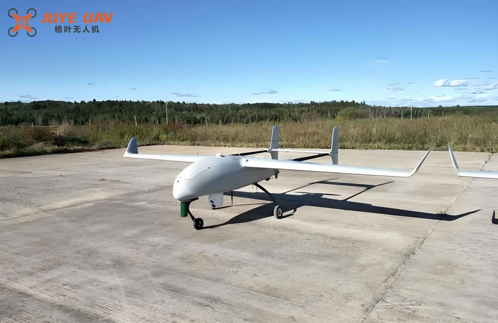
Fixed-wing drones have become essential in modern military and civilian applications due to their endurance and speed. However, trajectory planning for such drones is challenging because of complex dynamics, stringent control constraints, and the need for real-time obstacle avoidance. Unlike rotary-wing drones, fixed-wing drones cannot hover and must maintain forward flight, making real-time planning critical.
Over the past decades, various methods have been applied to path planning: graph search, artificial potential fields, and swarm intelligence. These methods often ignore the specific dynamics of fixed-wing drones, leading to paths that are not flyable. On the other hand, numerical optimization methods (nonlinear programming and sequential convex optimization) can handle dynamics but suffer from convergence issues and high computational cost.
To address these limitations, we propose a novel two-step framework. First, we design a path using Dubins curves that explicitly consider the minimum turn radius derived from the drone’s control constraints. Second, we formulate a velocity optimization problem that minimizes flight time. By introducing new variables and an exact convex relaxation, we transform the non-convex problem into a single convex optimization problem, eliminating iterative processes. Theoretical analysis proves that the relaxed constraint is active at the optimum, ensuring solution consistency.
2. Problem Description
A fixed-wing drone operates in a horizontal plane with obstacles (circular regions). The drone must travel from an initial state (position, velocity, heading) to a terminal state while avoiding obstacles and respecting dynamics and control bounds. The dynamics include lift, drag, thrust, and turning constraints. The key constraints are:
- Control constraints: thrust limits (\(T_{\min} \le T \le T_{\max}\)), lift coefficient limits (\(0 \le C_L \le C_{L,\max}\)), and bank angle limits (\(|\sigma| \le \sigma_{\max}\)).
- Velocity constraints: \(v_{\min} \le v \le v_{\max}\).
- Obstacle avoidance: \((x – x_{Oi})^2 + (y – y_{Oi})^2 \ge r_{Oi}^2\).
The objective is to minimize flight time. We decompose the problem into path planning (geometric) and velocity optimization along that path.
3. Path Planning Using Dubins Paths
3.1 Dubins Path Generation with Drone Constraints
Dubins paths consist of circular arcs and straight segments (CSC or CCC). For fixed-wing drones, we primarily use CSC paths (LSL, LSR, RSL, RSR). The minimum turn radius is derived from the balance of lift and centrifugal force:
$$ L \cos \sigma = mg, \quad L \sin \sigma = m v^2 / r. $$
Considering the maximum lift due to \(C_{L,\max}\) and the maximum bank angle \(\sigma_{\max}\), the maximum lateral lift is:
$$ (L \sin \sigma)_{\max} = \min\left\{ \sqrt{L_{\max}^2 – (mg)^2}, \; mg \tan \sigma_{\max} \right\}, $$
where \(L_{\max} = 0.5 \rho v^2 S C_{L,\max}\). Consequently, the minimum turn radius is:
$$ r_{\min} = \frac{m v^2}{(L \sin \sigma)_{\max}(v)}. $$
Given initial and terminal states \((x_0, y_0, \psi_0, r_0)\) and \((x_f, y_f, \psi_f, r_f)\), we compute the Dubins path using analytic geometry.
3.2 Single-Obstacle Avoidance
If the direct Dubins path intersects an obstacle, we select an intermediate waypoint on the boundary of the obstacle. For example, if the obstacle center \(O\) lies below the straight segment, we choose waypoint \(A\) above. The waypoint’s heading is the same as the segment’s azimuth. Its turn radius is taken as:
$$ r_A = \max\left\{ r_O, \; \frac{m v_c^2}{(L \sin \sigma)_{\max}(v_c)} \right\}, $$
where \(v_c\) is a reference speed (we search from \(v_{\max}\) downward until a feasible Dubins path is obtained). A typical step size \(\Delta v = 0.2\, \text{m/s}\) is used.
3.3 Multi-Obstacle Environment
We extend the single-obstacle method iteratively. First, find the direct Dubins path. For each unsafe segment, identify the nearest obstacle and insert a waypoint. Repeat until all segments are safe. The algorithm is summarized in the following steps:
- Input: drone parameters, start/end states, obstacle data.
- Compute direct Dubins path.
- Check safety; if safe, go to step 5.
- For each unsafe segment, find the nearest obstacle, insert a waypoint (as above), update path, return to step 3.
- Output: path coordinates, heading, curvature.
The computational complexity is low, requiring only geometric calculations and logic.
4. Exact Convex Relaxation for Velocity Optimization
4.1 Velocity Optimization Problem
Given the path, we optimize the velocity profile to minimize flight time. Use \(s\) (arc length) as independent variable and define \(\bar{v}=v^2\). The dynamics become:
$$ \frac{d\bar{v}}{ds} = \frac{2T}{m} – \frac{c_0 \rho S}{m} \bar{v} – \frac{4c_1}{m \rho S} \frac{L^2}{\bar{v}}. $$
Path tracking constraints:
$$ L \cos \sigma = mg, \quad L \sin \sigma = k m \bar{v}, $$
where \(k\) is the path curvature. The goal is to minimize flight time \(t_f = \int_{s_0}^{s_f} 1/v \, ds\). We replace this with an equivalent linear objective: minimize \(-\int \bar{v} \, ds\).
The resulting problem (P0) is non-convex due to the term \(L^2/\bar{v}\) and the product constraints.
4.2 Convexification via Exact Relaxation
Define new control variables:
$$ u_1 = L \cos \sigma, \quad u_2 = L \sin \sigma, \quad u_3 = \frac{L^2}{\bar{v}}. $$
Then the dynamics become linear:
$$ \frac{d\bar{v}}{ds} = \frac{2T}{m} – \frac{c_0 \rho S}{m} \bar{v} – \frac{4c_1}{m \rho S} u_3. $$
The path constraints become linear equalities:
$$ u_1 = mg, \quad u_2 = k m \bar{v}. $$
The non-convex equality constraint relating these variables is:
$$ u_1^2 + u_2^2 = u_3 \bar{v}. $$
We relax this to a convex inequality:
$$ u_1^2 + u_2^2 \le u_3 \bar{v}. $$
To ensure the relaxation is exact (i.e., the constraint is active at the optimum), we modify the objective by adding a regularization term:
$$ J_3 = -\int_{s_0}^{s_f} \bar{v} \, ds + c_r \int_{s_0}^{s_f} u_3 \, ds, $$
where \(c_r\) is a small positive coefficient. Theorem 2 proves that under mild assumptions (thrust and velocity bounds not simultaneously active), the inequality constraint holds with equality almost everywhere. The proof uses optimal control theory (Hamiltonian, Lagrange multipliers, complementary slackness).
4.3 Solution Strategy
After discretization (e.g., Euler method with 101 points), the resulting problem (P2) is a convex optimization problem (second-order cone program) that can be solved by interior-point solvers like ECOS. No iterative loop is needed, guaranteeing convergence in a single shot. From the solution we recover the velocity \(v = \sqrt{\bar{v}}\), thrust \(T\), lift coefficient \(C_L\), and bank angle \(\sigma\).
5. Simulation Results
5.1 Multi-Obstacle Environment
We simulated a fixed-wing drone with parameters given in Table 1. The drone starts at (0 m, 0 m) with speed 30 m/s and heading 0°, ends at (500 m, 100 m) with 36 m/s. Two obstacles: O1 (center (180,90), radius 100 m); O2 (center (330,20), radius 60 m).
Table 1: Fixed-wing drone parameters
| Parameter | Value | Parameter | Value |
|---|---|---|---|
| m (kg) | 11.5 | \(v_{\max}\) (m/s) | 40 |
| S (m²) | 0.84 | \(v_{\min}\) (m/s) | 25 |
| \(c_0\) | 0.0339 | \(T_{\max}\) (N) | 100 |
| \(c_1\) | 0.1834 | \(T_{\min}\) (N) | 10 |
| \(C_{L,\max}\) | 0.6083 | \(\sigma_{\max}\) (deg) | 60 |
The path planning process is illustrated in our simulations: the first Dubins path passed through both obstacles; we inserted waypoint A for O1, then waypoint B for O2, obtaining a safe path I-A-B-F. Notably, during the A-B segment, the initial reference speed \(v_c=40\) m/s gave a turn radius too large (94.17 m) causing intersection of turning circles; searching with step 0.2 m/s down to 37.2 m/s (radius 81.44 m) yielded a feasible Dubins path. This shows the necessity of the search process.
Velocity optimization using ECOS (101 points) produced the profiles shown in Figure 7 of the original paper. The velocity and thrust respect all constraints: acceleration uses maximum thrust, deceleration uses minimum thrust, and steady flight balances thrust with drag. Importantly, the regularized objective ensures that the relaxed inequality is active throughout the trajectory (Figure 8b), validating Theorem 2.
5.2 Unknown Obstacle Environment
We tested online replanning in an unknown environment. The drone starts at (0 m, 50 m, 30 m/s, 0°) and aims for (800 m, 200 m, 36 m/s, 0°). Two hidden obstacles: O1 (center (280,160), radius 140 m); O2 (center (600,120), radius 90 m). Detection range is 100 m. The drone follows the initial path until it detects O1 at point A, then replans; later detects O2 at point B and replans again. The final path avoids both obstacles. Computation times for the initial plan and two updates were 12.18 ms, 11.79 ms, and 11.89 ms, respectively, well within real-time requirements.
5.3 Adaptability and Real-Time Performance
We ran 101 test scenarios with different starting positions around the target. The obstacles are given in Table 2.
Table 2: Obstacle parameters
| Obstacle | \(x_O\) (m) | \(y_O\) (m) | \(r_O\) (m) |
|---|---|---|---|
| 1 | 280 | 90 | 105 |
| 2 | 640 | 160 | 140 |
| 3 | 500 | -180 | 120 |
| 4 | 200 | -140 | 70 |
Our method succeeded in all 101 cases. We compared computational efficiency with two alternative methods: nonlinear programming (GPOPS-II, using SNOPT) and sequential convex optimization (with ECOS). The results are summarized in Table 3.
Table 3: Computational efficiency comparison across 101 cases
| Method | Average iterations | Average computation time (ms) |
|---|---|---|
| Nonlinear programming [24] | 11.53 | 2541.52 |
| Sequential convex optimization [25] | 6.62 | 435.48 |
| Proposed method | 1 (no iteration) | 12.60 |
Our method is over 200 times faster than nonlinear programming and over 30 times faster than sequential convex optimization, while guaranteeing feasibility and optimality (up to the regularization term).
6. Conclusion
We have developed a real-time trajectory planning framework for fixed-wing drones by combining Dubins-based path planning with an exact convex relaxation for velocity optimization. The key contributions are:
- A path planning method that respects the minimum turn radius of the fixed-wing drone derived from its control constraints, ensuring flyability in multi-obstacle environments.
- A convexification technique that transforms the non-convex velocity optimization into a single convex problem using new variables and a regularized objective, with theoretical proof that the relaxed constraint is active at the optimum.
- Computational efficiency: the entire process takes only tens of milliseconds, enabling online replanning in unknown environments.
Simulation results demonstrate that the method reliably generates obstacle-free paths and optimal velocity profiles, outperforming conventional nonlinear and sequential convex optimization methods. This approach is well-suited for real-world fixed-wing drone missions such as reconnaissance, communication relay, and combat assessment.