
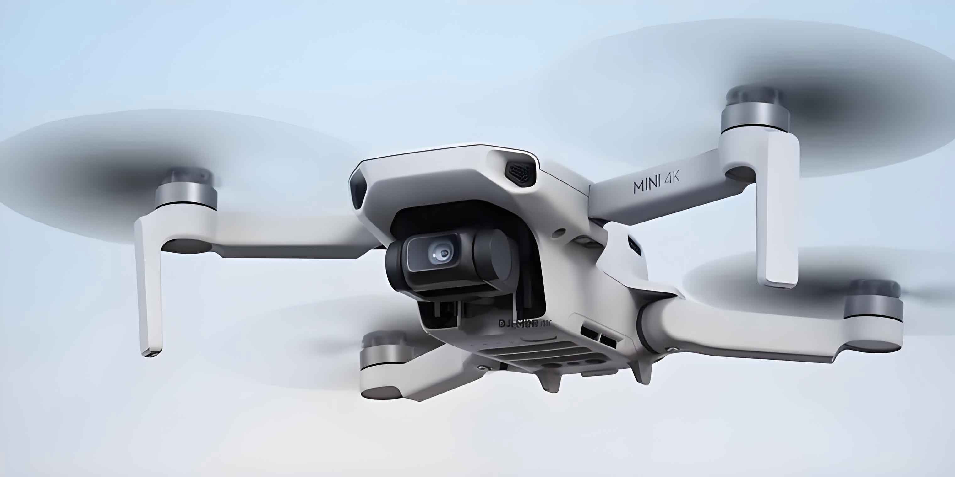
In the context of rapidly evolving wireless communication technologies, the integration of unmanned aerial vehicle (UAV) systems into cellular networks has become a critical research area. The ability of an unmanned aerial vehicle to navigate autonomously while maintaining reliable connectivity with ground base stations is essential for a wide range of applications, including delivery services, surveillance, and emergency response. This article presents a comprehensive study on intelligent path navigation for cellular-connected unmanned aerial vehicles, leveraging the synergy between radio map reconstruction and deep reinforcement learning. The proposed framework reconstructs a high-fidelity radio map from sparse measurements and subsequently employs a dueling double deep Q-network to optimize the flight trajectory under connectivity constraints. Extensive simulations demonstrate that the reconstructed radio map enables the unmanned aerial vehicle to learn near-optimal paths with significantly lower communication outage probability, while reducing the need for costly real-world trial-and-error exploration.
Introduction and Motivation
The deployment of unmanned aerial vehicles as aerial communication platforms has attracted significant attention due to their flexibility, mobility, and ability to provide on-demand connectivity. In sixth-generation (6G) networks, the convergence of communication and sensing is expected to unlock new capabilities for unmanned aerial vehicles, particularly in the context of path navigation and environment mapping. However, the inherent challenges of complex urban environments, such as signal blockage, multipath fading, and dynamic interference, make it difficult to guarantee reliable communication links between the unmanned aerial vehicle and ground base stations.
Traditional path navigation methods for unmanned aerial vehicles often rely on global positioning system signals or pre-defined maps, which may not capture the actual radio frequency environment. Furthermore, conventional optimization-based approaches require accurate channel models and full knowledge of the propagation environment, which are rarely available in practice. To overcome these limitations, radio map reconstruction has emerged as a promising technique. A radio map, also known as a channel gain map or outage probability map, provides spatial information about the expected communication quality at every location in the environment. By reconstructing this map from limited measurements, an unmanned aerial vehicle can plan its trajectory in advance, avoiding regions of high outage probability and ensuring reliable connectivity throughout the mission.
The main contributions of this article are twofold. First, we introduce two novel radio map reconstruction algorithms based on untrained network priors: the deep image prior-based radio map construction (RMC-DIP) and the deep denoising regularized radio map construction (RMC-DDR). These algorithms exploit the structural inductive bias of convolutional neural networks to reconstruct high-resolution radio maps from sparse samples without requiring any labeled training data. Second, we formulate the unmanned aerial vehicle path navigation problem as a Markov decision process and solve it using a dueling double deep Q-network (D3QN). The reconstructed radio map serves as a virtual environment for offline training, allowing the unmanned aerial vehicle to learn an optimal policy before executing its mission. Simulation results show that the proposed method achieves a communication outage time very close to that of the ideal case where the true channel map is available, while significantly outperforming traditional interpolation-based reconstruction methods.
System Model and Problem Formulation
We consider a scenario where a single unmanned aerial vehicle flies within a three-dimensional cuboid region denoted by \(\mathcal{V} = [x_1, x_2] \times [y_1, y_2] \times [z_1, z_2]\). The position of the unmanned aerial vehicle at discrete time slot \(m\) is denoted by \(\mathbf{l}_m = (x_m, y_m, z_m)\). The mission starts at the initial position \(\mathbf{l}_I\) and ends at a fixed final position \(\mathbf{l}_F\). The total flight time is divided into \(M\) slots, each of duration \(\Delta t\), such that \(T = M \Delta t\). The unmanned aerial vehicle moves with a constant speed \(v_s\), and the movement direction is chosen from a discrete action space.
There are \(C\) ground base stations in the region, each transmitting with power \(P_c\) for \(c = 1, 2, \ldots, C\). The received signal power at the unmanned aerial vehicle from base station \(c\) is expressed as:
\[
p_c(\mathbf{l}_m) = P_c \beta_c(\mathbf{l}_m) G_c(\mathbf{l}_m) |\tilde{h}_c(m)|^2,
\]
where \(\beta_c(\mathbf{l}_m)\) is the large-scale channel gain, \(G_c(\mathbf{l}_m)\) is the antenna gain, and \(\tilde{h}_c(m)\) represents small-scale fading. The unmanned aerial vehicle is associated with the base station that provides the strongest signal at each time slot. Define the association index \(c'(m) \in \{1, \ldots, C\}\). The signal-to-interference ratio (SIR) at time slot \(m\) is given by:
\[
\mathrm{SIR}(\mathbf{l}_m) = \frac{p_{c'(m)}(\mathbf{l}_m)}{\sum_{c \neq c'(m)} p_c(\mathbf{l}_m)}.
\]
An outage occurs when the SIR falls below a threshold \(\gamma_{\mathrm{th}}\). The outage probability at position \(\mathbf{l}_m\) is thus:
\[
P_{\mathrm{out}}(\mathbf{l}_m, c'(m)) = \Pr\left[ \mathrm{SIR}(\mathbf{l}_m) < \gamma_{\mathrm{th}} \right].
\]
The total outage time during the mission is computed as:
\[
T_{\mathrm{out}} = \sum_{m=1}^{M} P_{\mathrm{out}}(\mathbf{l}_m, c'(m)) \Delta t.
\]
The weighted time cost is defined as the sum of the mission completion time and the outage time with weights \(\alpha\) and \(\beta\), respectively:
\[
T_s = \alpha T + \beta T_{\mathrm{out}}.
\]
Since maintaining a reliable communication link is paramount, the weight \(\beta\) is set to a large constant. The energy consumption of the unmanned aerial vehicle is dominated by the propulsion power. For a fixed-wing unmanned aerial vehicle flying at constant speed \(v\) and zero acceleration, the propulsion power is:
\[
P_{\mathrm{prop}} = c_1 v^3 + \frac{c_2}{v},
\]
where \(c_1\) and \(c_2\) are constant parameters depending on air density, aircraft weight, and wing area. The total flight energy is then \(E_f = T P_{\mathrm{prop}}\). The optimization goal is to minimize the total energy consumption while satisfying the connectivity constraint, which is equivalent to minimizing the weighted time cost \(T_s\). We convert this minimization problem into a maximization problem by defining the reward function as the negative weighted time cost per step.
Radio Map Reconstruction with Untrained Network Priors
The first key component of our framework is the reconstruction of a high-resolution radio map from a limited number of sparse measurements. The unmanned aerial vehicle samples \(N\) random locations in the target area and computes the outage probability at each location using the channel model described above. These sampled values form a low-resolution map \(\mathbf{y}_0\) with dimensions \((m/s) \times (n/s)\), where \(m \times n\) is the desired resolution and \(s\) is the downsampling factor.
Problem Formulation
The radio map reconstruction problem can be cast as an energy minimization problem:
\[
\min_{\mathbf{y}} \; \frac{1}{2} \| \mathbf{y}_0 – \mathcal{H} \mathbf{y} \|_2^2 + \lambda \Phi(\mathbf{y}),
\]
where \(\mathcal{H}\) is a linear degradation operator, \(\Phi(\mathbf{y})\) is a regularization term, and \(\lambda\) is a trade-off parameter. Traditional methods hand-craft the regularizer using priors such as smoothness or sparsity. In contrast, we leverage the implicit prior captured by a deep convolutional network.
RMC-DIP: Deep Image Prior Approach
The deep image prior method replaces the explicit regularization by the structure of a randomly initialized convolutional generator network. We represent the reconstructed map as the output of the network:
\[
\mathbf{y} = f_{\boldsymbol{\theta}}(\mathbf{z}),
\]
where \(\mathbf{z}\) is a fixed random tensor and \(\boldsymbol{\theta}\) are the network parameters. The optimization problem becomes:
\[
\min_{\boldsymbol{\theta}} \; \frac{1}{2} \| \mathbf{y}_0 – \mathcal{H} f_{\boldsymbol{\theta}}(\mathbf{z}) \|_2^2.
\]
The network is trained using gradient descent without any external data. The iterative process progressively refines the output to match the observed samples while maintaining the natural image statistics imposed by the network architecture. The pseudo-code of the RMC-DIP algorithm is summarized in Table 1.
| Step | Description |
|---|---|
| 1 | Initialize matrix \(\mathbf{R}\), downsampling factor \(s\), upsampling factor \(u\), deep convolutional network \(f_{\boldsymbol{\theta}}\) with random parameters. |
| 2 | Generate a random input tensor \(\mathbf{z}\) with the same spatial size as the desired output. |
| 3 | Set total iterations \(T\). |
| 4 | For \(t = 1\) to \(T\) do: |
| 5 | Compute the output \(\mathbf{y} = f_{\boldsymbol{\theta}}(\mathbf{z})\). |
| 6 | Calculate the loss \(\mathcal{L} = \| \mathbf{y}_0 – \mathcal{H} \mathbf{y} \|_2^2\). |
| 7 | Update \(\boldsymbol{\theta}\) by backpropagation to minimize \(\mathcal{L}\). |
| 8 | End for |
| 9 | Return the reconstructed map \(\mathbf{y}\). |
This approach eliminates the need for labeled training data and can be directly applied to any new environment without re-training on a dataset. The output of the RMC-DIP algorithm is a radio map in which each pixel represents the outage probability at that spatial location.
RMC-DDR: Deep Denoising Regularization
Although the deep image prior already offers strong performance, we further improve upon it by integrating a denoising-based regularization. The idea of regularization by denoising (RED) is to define the regularizer using a denoising function \(f(\cdot)\):
\[
\Phi(\mathbf{y}) = \frac{1}{2} \mathbf{y}^T \left( \mathbf{y} – f(\mathbf{y}) \right).
\]
Combining this with the deep image prior representation yields the RMC-DDR algorithm. The optimization problem is rewritten as:
\[
\min_{\boldsymbol{\theta}} \; \frac{1}{2} \| \mathbf{y}_0 – \mathcal{H} f_{\boldsymbol{\theta}}(\mathbf{z}) \|_2^2 + \frac{\lambda}{2} f_{\boldsymbol{\theta}}(\mathbf{z})^T \left( f_{\boldsymbol{\theta}}(\mathbf{z}) – f(f_{\boldsymbol{\theta}}(\mathbf{z})) \right).
\]
Since differentiating the denoiser is intractable for most denoising algorithms, we employ the alternating direction method of multipliers (ADMM) to solve the problem. By introducing an auxiliary variable \(\mathbf{y}\) and a Lagrange multiplier vector \(\mathbf{v}\), we transform the constrained problem into an augmented Lagrangian form. The ADMM iterates over three steps: updating the network parameters \(\boldsymbol{\theta}\), updating the auxiliary variable \(\mathbf{y}\), and updating the multiplier \(\mathbf{v}\). The procedure is sketched in Table 2.
| Step | Update Rule |
|---|---|
| Input | Degraded map \(\mathbf{y}_0\), degradation operator \(\mathcal{H}\), noise level \(\varepsilon\), regularization parameter \(\lambda\), ADMM penalty \(\mu\). |
| Initialization | Set \(k=0\), initialize \(\boldsymbol{\theta}_0\), \(\mathbf{y}_0\), \(\mathbf{v}_0\). |
| Repeat | Update \(\boldsymbol{\theta}_{k+1}\) by minimizing the augmented Lagrangian with fixed \(\mathbf{y}_k\) and \(\mathbf{v}_k\). |
| Update \(\mathbf{y}_{k+1}\) by solving a denoising-based proximal problem with fixed \(\boldsymbol{\theta}_{k+1}\) and \(\mathbf{v}_k\). | |
| Update \(\mathbf{v}_{k+1} = \mathbf{v}_k + \mu(\mathbf{y}_{k+1} – f_{\boldsymbol{\theta}_{k+1}}(\mathbf{z}))\). | |
| Until | Convergence criterion is satisfied. |
| Output | Reconstructed map \(\mathbf{y}\). |
The RMC-DDR method combines the expressive power of deep neural networks with the stabilizing effect of explicit denoising regularization. As a result, it achieves better performance in terms of peak signal-to-noise ratio (PSNR), structural similarity index (SSIM), and normalized mean squared error (NMSE) compared to both the RMC-DIP and traditional interpolation methods, especially when the sampling rate is low or the data is corrupted by noise.
UAV Path Navigation via Deep Reinforcement Learning
Once the radio map is reconstructed offline, the unmanned aerial vehicle can utilize it to plan its path ahead of time. We model the path navigation problem as a Markov decision process (MDP) defined by the tuple \((\mathcal{S}, \mathcal{A}, \mathcal{P}, \mathcal{R})\). The state space \(\mathcal{S}\) contains all possible positions of the unmanned aerial vehicle inside the navigation region. The action space \(\mathcal{A}\) consists of four discrete movement directions (forward, backward, left, right) in the horizontal plane, while the altitude is assumed to be fixed for simplicity. The transition probability \(\mathcal{P}\) is deterministic given the action. The reward function is designed to encourage fast arrival and penalize communication outages:
\[
R(\mathbf{l}_m) = -1 – \mu P_{\mathrm{out}}(\mathbf{l}_m, c'(m)),
\]
where \(\mu\) is a large penalty coefficient for outage occurrences. The negative constant \( -1 \) at each step reflects the time cost, motivating the unmanned aerial vehicle to reach the destination as quickly as possible. The cumulative discounted reward is:
\[
G = \sum_{m=1}^{M} \gamma^{m-1} R(\mathbf{l}_m),
\]
where \(\gamma \in (0,1]\) is the discount factor. The objective is to find a policy \(\pi\) that maximizes the expected cumulative reward.
D3QN Algorithm
To solve the MDP, we use the dueling double deep Q-network (D3QN) architecture. The D3QN combines two key improvements over the standard deep Q-network: double Q-learning to reduce overestimation bias and a dueling network structure that separately estimates the state value and the action advantage. The Q-value is computed as:
\[
Q(s, a; \boldsymbol{\theta}, \boldsymbol{\phi}) = V(s; \boldsymbol{\phi}) + A(s, a; \boldsymbol{\theta}) – \frac{1}{|\mathcal{A}|} \sum_{a’} A(s, a’; \boldsymbol{\theta}),
\]
where \(\boldsymbol{\phi}\) and \(\boldsymbol{\theta}\) are the parameters of the value and advantage streams, respectively. The training process uses experience replay and a target network with periodic updates. The pseudo-code of the D3QN-based path navigation algorithm is presented in Table 3.
| Step | Description |
|---|---|
| 1 | Use a radio map reconstruction algorithm to obtain the reconstructed outage probability map. |
| 2 | Initialize the current Q-network with parameters \(\boldsymbol{\theta}\), and the target Q-network with parameters \(\boldsymbol{\theta}’ = \boldsymbol{\theta}\). Set total episodes \(E\), per-episode steps \(M\), discount factor \(\gamma\), learning rate \(\eta\), target network update frequency \(F\), and mini-batch size \(B\). |
| 3 | Initialize replay buffer \(\mathcal{D}\). |
| 4 | For each episode \(e = 1, \ldots, E\): |
| 5 | Reset the environment to the initial position \(\mathbf{l}_I\). Get current state \(s\). Set \(done = \text{False}\). |
| 6 | For each step \(t = 1, \ldots, M\) and while \(done = \text{False}\): |
| 7 | Select action \(a\) according to an \(\epsilon\)-greedy policy based on \(Q(s, a; \boldsymbol{\theta})\). |
| 8 | Execute action \(a\), observe new position \(s’\), obtain outage probability from the reconstructed map, and compute reward \(R = -1 – \mu P_{\mathrm{out}}\). |
| 9 | If \(s’\) equals the final position \(\mathbf{l}_F\), set \(done = \text{True}\). |
| 10 | Store transition \((s, a, R, s’, done)\) in \(\mathcal{D}\). |
| 11 | Sample a random mini-batch of \(B\) transitions from \(\mathcal{D}\). |
| 12 | Compute target Q-value using the target network: \(y_j = R_j + \gamma \max_{a’} Q(s_j’, a’; \boldsymbol{\theta}’)\) for non-terminal states. |
| 13 | Compute the mean squared error loss and update \(\boldsymbol{\theta}\) via gradient descent. |
| 14 | Every \(F\) steps, set \(\boldsymbol{\theta}’ = \boldsymbol{\theta}\). |
| 15 | Set \(s = s’\). |
| 16 | End for |
| 17 | End for |
| 18 | Return the trained Q-network for path selection. |
The key advantage of this offline training scheme is that the unmanned aerial vehicle does not need to interact with the physical environment during the learning phase. Instead, it queries the reconstructed radio map to obtain the outage probability at any candidate position, which drastically reduces the time and cost of collecting real-world data. Moreover, the trained policy can be transferred to the actual unmanned aerial vehicle with minimal performance loss, as the reconstructed map captures the essential spatial variability of the communication channel.
Simulation Results and Analysis
We conduct a series of simulations to evaluate the proposed radio map reconstruction and path navigation algorithms. The simulated environment is a \(2 \times 2\) km area with high-rise buildings and two ground base stations positioned at predefined locations. The building distribution follows the ITU statistical model with parameters \(\alpha_{bd} = 0.3\), \(\beta_{bd} = 300\), \(\gamma_{bd} = 50\) m, and a maximum building height of 90 m. The large-scale path loss is modeled using the 3GPP urban macro (UMa) model, and small-scale fading is simulated as Rayleigh fading for non-line-of-sight (NLoS) links and Rician fading with a 15 dB factor for line-of-sight (LoS) links. The ground base station antenna height is set to 25 m. The target radio map has a resolution of \(201 \times 201\) pixels.
For the reconstruction experiments, we compare the proposed RMC-DIP and RMC-DDR algorithms against a traditional Kriging algorithm based on a spherical variogram model. The reconstruction quality is measured by PSNR, SSIM, and NMSE. Table 4 summarizes the results at different sampling rates (1%, 5%, 10%, and 25%).
| Sampling Rate | PSNR (dB) | SSIM | NMSE | ||||||
|---|---|---|---|---|---|---|---|---|---|
| Kriging | RMC-DIP | RMC-DDR | Kriging | RMC-DIP | RMC-DDR | Kriging | RMC-DIP | RMC-DDR | |
| 1% | 10.69 | 18.19 | 18.20 | 0.011 | 0.448 | 0.464 | 0.254 | 0.157 | 0.156 |
| 5% | 10.54 | 20.08 | 20.35 | 0.005 | 0.640 | 0.689 | 0.263 | 0.102 | 0.095 |
| 10% | 10.36 | 21.66 | 22.07 | 0.011 | 0.772 | 0.788 | 0.274 | 0.071 | 0.064 |
| 25% | 10.70 | 23.86 | 24.24 | 0.012 | 0.863 | 0.867 | 0.238 | 0.042 | 0.039 |
The table clearly demonstrates the superiority of the untrained-prior-based methods over the Kriging approach. At a 25% sampling rate, the RMC-DDR algorithm achieves a PSNR gain of 13.54 dB over Kriging and 0.38 dB over RMC-DIP. Similarly, the SSIM values obtained by the proposed methods are over an order of magnitude higher than those of Kriging, indicating that the structural information of the radio map is much better preserved. The NMSE is correspondingly reduced, confirming the accuracy of the reconstructed maps.
To further analyze the convergence behavior of the reconstruction algorithms, we plot the PSNR and SSIM values against the number of iterations for different downsampling factors (SF10, SF5, SF3, SF2). The results show that the RMC-DDR algorithm converges much faster and reaches higher final PSNR and SSIM values than the RMC-DIP algorithm across all downsampling factors. For instance, with SF2, the RMC-DDR attains a PSNR above 30 dB within 200 iterations, while the RMC-DIP requires more than 400 iterations to approach a similar value. This improvement is attributed to the additional denoising regularizer that stabilizes the gradient updates and prevents the network from overfitting to the sparse measurements.
In the path navigation experiments, we compare the trajectories learned under the reconstructed radio map with those learned directly in the actual environment. The unmanned aerial vehicle begins at a random position and aims to reach a fixed target position. The D3QN algorithm is trained with a total of 5000 episodes. The performance metrics include the total outage time, the probability of successfully reaching the destination, the average episode reward, and the flight energy consumption.
Figure 1 (not shown here) visually presents the obtained trajectories. The path planned using the reconstructed radio map closely follows the path obtained with the actual map, demonstrating that the reconstructed map preserves the essential connectivity features of the environment. The unmanned aerial vehicle naturally tends to pass through regions with high coverage (equivalently low outage probability) and avoids areas shadowed by buildings. This behavior results in a reliable communication link throughout the mission.
Table 5 lists the total outage time averaged over the successful episodes for different downsampling factors and reconstruction methods.
| Downsampling Factor | Kriging | RMC-DIP | RMC-DDR |
|---|---|---|---|
| 2 | 1.8 s | 0.9 s | 0.8 s |
| 4 | 2.5 s | 1.3 s | 1.1 s |
| 8 | 3.7 s | 2.1 s | 1.9 s |
| 16 | 5.2 s | 3.0 s | 2.7 s |
As expected, the outage time increases with the downsampling factor because the reconstructed map becomes less accurate. However, at every downsampling factor, the proposed RMC-DIP and RMC-DDR algorithms yield significantly lower outage times than Kriging, and the RMC-DDR performs slightly better than RMC-DIP. These results confirm that a more accurate radio map directly enables better path decisions and reduces the risk of communication failures.
The probability of successfully reaching the destination is shown in Table 6 for different training episodes. The results demonstrate that after about 3000 episodes, the unmanned aerial vehicle learns a stable policy that consistently guides it to the target under the connectivity constraint. The success probability with RMC-DIP at a downsampling factor of 2 is almost as high as that obtained in the actual environment, indicating that the reconstructed map is sufficiently accurate for practical purposes.
| Training Episodes | Actual Environment | RMC-DIP (SF2) | RMC-DIP (SF4) | RMC-DIP (SF16) | Kriging (SF4) |
|---|---|---|---|---|---|
| 1000 | 0.45 | 0.40 | 0.35 | 0.20 | 0.15 |
| 2000 | 0.78 | 0.72 | 0.64 | 0.42 | 0.30 |
| 3000 | 0.95 | 0.91 | 0.85 | 0.62 | 0.50 |
| 5000 | 0.98 | 0.96 | 0.92 | 0.71 | 0.58 |
The average cumulative reward per episode is displayed in Table 7. The reward values are negative due to the per-step penalty of \(-1\) and the additional outage penalty. As training proceeds, the moving average reward increases (becomes less negative), indicating that the agent learns to shorten the path and avoid outage regions. The reward obtained with the actual environment is the highest, followed by RMC-DIP with downsampling factor 2, then 4, and finally 16. Even the RMC-DIP with downsampling factor 8 outperforms the Kriging method with factor 4, which further validates the effectiveness of our reconstruction approach.
| Method | Downsampling Factor | Average Reward |
|---|---|---|
| Actual environment | – | -285 |
| RMC-DIP | 2 | -310 |
| RMC-DIP | 4 | -365 |
| RMC-DIP | 8 | -440 |
| RMC-DIP | 16 | -520 |
| Kriging | 4 | -590 |
Finally, we compare the flight energy consumption of the unmanned aerial vehicle when following the learned path under different radio maps. The propulsion energy is calculated using the formula \(E_f = P_{\mathrm{prop}} T\). Since the unmanned aerial vehicle flies at constant speed, the energy is directly proportional to the total flight time. The results indicate that the energy consumption for paths learned with our reconstructed maps is only slightly higher than the minimum energy required for a straight-line flight without connectivity constraints. The difference is about 2000 J, which is acceptable compared to the total average energy of about 7000 J. This demonstrates that the unmanned aerial vehicle can maintain good connectivity without sacrificing much energy efficiency.
Conclusion and Future Work
This article presented a comprehensive framework for intelligent path navigation of cellular-connected unmanned aerial vehicles based on radio map reconstruction and deep reinforcement learning. The proposed radio map reconstruction algorithms, RMC-DIP and RMC-DDR, leverage untrained network priors to recover high-resolution outage probability maps from sparse samples, eliminating the need for large labeled datasets. The D3QN-based path navigation algorithm then utilizes the reconstructed map as an offline virtual environment to learn an optimal trajectory under connectivity constraints. Extensive simulations demonstrated that the reconstructed maps closely approximate the real environment, enabling the unmanned aerial vehicle to achieve near-optimal paths with low outage time and high energy efficiency.
Several avenues for future work are worth exploring. First, the reconstruction algorithms can be enhanced by incorporating more advanced generative models, such as generative adversarial networks, to further improve the accuracy and robustness of the radio maps. Second, the path navigation algorithm could be extended to multi-unmanned aerial vehicle scenarios, where cooperative planning and distributed learning would be required. Third, the assumption of constant altitude and horizontal-only movement can be relaxed to allow full three-dimensional trajectory optimization, which is more realistic for urban environments. Finally, the impact of dynamic environmental changes, such as moving obstacles or weather variations, could be incorporated by updating the radio map online during the mission. These extensions would bring the proposed framework closer to real-world deployment, ultimately enabling more reliable and intelligent unmanned aerial vehicle operations in future wireless networks.