
In highly adversarial battlefield environments, multi-fixed-wing UAV formations significantly enhance combat effectiveness and situational awareness. Coordinated execution of saturation attacks, distributed reconnaissance, and collaborative positioning demands robust formation control that ensures collision avoidance, velocity synchronization, and resilience against external disturbances, input saturation, and communication delays. In this work, we propose a novel formation control strategy based on extended state observers to address these challenges for fixed-wing UAV swarms.
1. Introduction
Fixed-wing UAV swarms have attracted extensive attention due to their ability to perform coordinated tasks such as multi-angle saturation attacks, simultaneous engagement of multiple targets, and comprehensive reconnaissance. Compared to single platforms, multiple fixed-wing UAVs operating in formation can achieve higher survivability and efficiency. However, the formation flight of fixed-wing UAVs faces several critical issues: collision avoidance, handling of external disturbances like gusts, input saturation constraints, and communication delays. Existing approaches can be categorized into optimization-based methods and rule-based methods. The potential function method, as a rule-based approach, is widely applied due to its clear physical meaning and flexibility in parameter selection. Moreover, extended state observers have been introduced to estimate and compensate for unknown disturbances in real time. In this paper, we integrate the potential function method with an anti-saturation compensator and time-varying communication delay handling to design a distributed formation controller for fixed-wing UAV systems. The main contributions are threefold:
- Design of an extended state observer to estimate external disturbances for fixed-wing UAVs, with proof of exponential convergence of estimation errors to a small neighborhood.
- A collision-avoidance saturated control strategy that combines potential functions with an anti-saturation compensator, explicitly considering input saturation and time-varying communication delays.
- Rigorous stability analysis showing asymptotic stability of the closed-loop system under strong connectivity of the communication graph and mild conditions on delays.
2. Problem Formulation
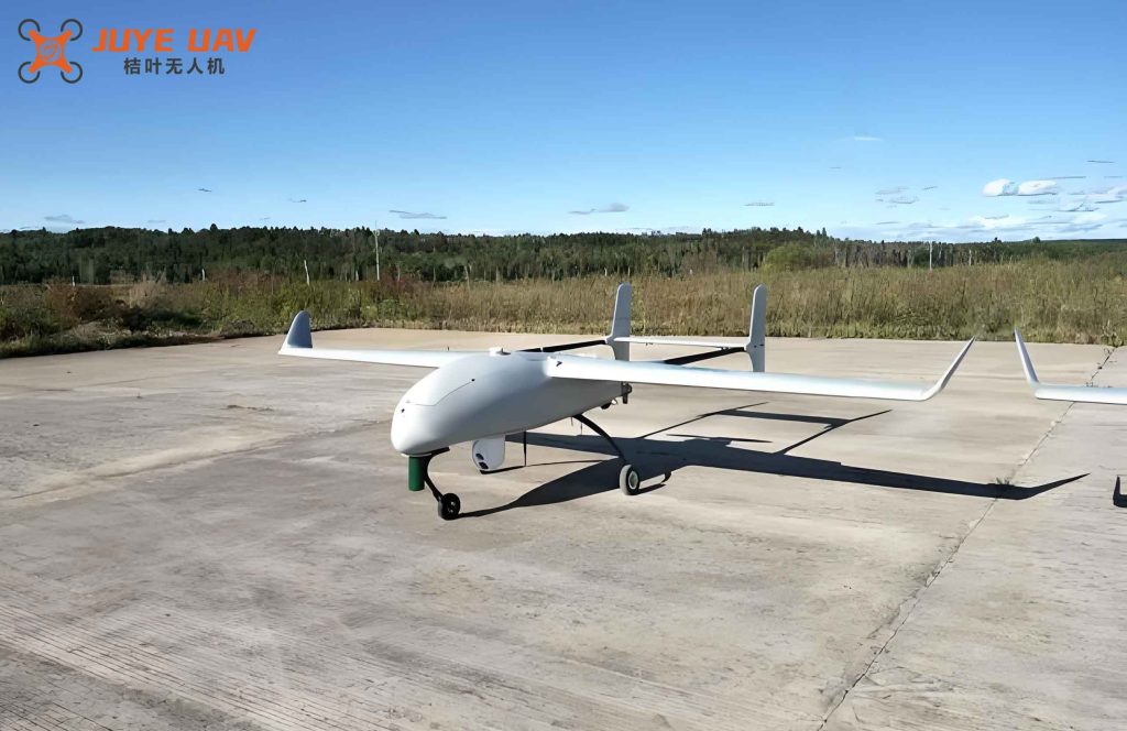
2.1 Fixed-wing UAV Dynamics
Consider a formation of \(n\) fixed-wing UAVs. For the \(i\)-th fixed-wing UAV, the kinematic equations are:
$$
\begin{aligned}
\dot{x}_i &= V_i \cos\chi_i \cos\gamma_i, \\
\dot{y}_i &= V_i \sin\chi_i \cos\gamma_i, \\
\dot{z}_i &= V_i \sin\gamma_i,
\end{aligned}
$$
where \(\mathbf{p}_i = [x_i, y_i, z_i]^\top\) denotes the position vector, \(V_i\) the airspeed, \(\chi_i\) the heading angle, and \(\gamma_i\) the flight path angle. The dynamic equations are given by:
$$
\begin{aligned}
\dot{V}_i &= \frac{T_i – D_i + d_{V_i}}{m_i} – g\sin\gamma_i, \\
\dot{\chi}_i &= \frac{L_i \sin\phi_i + d_{\chi_i}}{m_i V_i \cos\gamma_i}, \\
\dot{\gamma}_i &= \frac{L_i \cos\phi_i – m_i g\cos\gamma_i + d_{\gamma_i}}{m_i V_i},
\end{aligned}
$$
where \(T_i\) is thrust, \(L_i\) lift, \(D_i\) drag, \(\phi_i\) the roll angle, \(m_i\) mass, \(g\) gravity, and \(d_{V_i}, d_{\chi_i}, d_{\gamma_i}\) unknown external disturbances. To facilitate controller design, define the control input \(\mathbf{F}_i = [T_i,\ L_i\sin\phi_i,\ L_i\cos\phi_i]^\top\), velocity \(\mathbf{v}_i = \dot{\mathbf{p}}_i\), and disturbance \(\mathbf{d}_{i0} = [d_{V_i}, d_{\chi_i}, d_{\gamma_i}]^\top\). Then the dynamics can be rewritten as:
$$
\begin{aligned}
\dot{\mathbf{p}}_i &= \mathbf{v}_i, \\
m_i \dot{\mathbf{v}}_i &= \boldsymbol{\alpha}_i + m_i \boldsymbol{\varepsilon}_i + \mathbf{R}_i \mathbf{F}_i + \mathbf{d}_i,
\end{aligned}
$$
with \(\mathbf{d}_i = \mathbf{R}_i \mathbf{d}_{i0}\), and matrices defined as:
$$
\boldsymbol{\alpha}_i = \begin{bmatrix} -D_i \cos\chi_i\cos\gamma_i \\ -D_i\sin\chi_i\cos\gamma_i \\ -D_i\sin\gamma_i \end{bmatrix},\quad
\boldsymbol{\varepsilon}_i = \begin{bmatrix}0\\0\\g\end{bmatrix},\quad
\mathbf{R}_i = \begin{bmatrix} \cos\chi_i\cos\gamma_i & -\sin\chi_i & -\sin\gamma_i\cos\chi_i \\ \sin\chi_i\cos\gamma_i & \cos\chi_i & -\sin\gamma_i\sin\chi_i \\ \sin\gamma_i & 0 & \cos\gamma_i \end{bmatrix}.
$$
Note that \(\mathbf{R}_i\) is invertible and \(\mathbf{R}_i^{-1} = \mathbf{R}_i^\top\).
2.2 Graph Theory
The information exchange among fixed-wing UAVs is modeled by a weighted directed graph \(\mathcal{G} = (\mathcal{V},\mathcal{E},\mathbf{C})\), where \(\mathcal{V} = \{1,2,\dots,n\}\) is the vertex set, \(\mathcal{E}\) the edge set, and \(\mathbf{C} = [c_{ij}] \in \mathbb{R}^{n\times n}\) the adjacency matrix. If there exists a directed edge from node \(j\) to node \(i\), then \(c_{ij} > 0\); otherwise \(c_{ij}=0\). The Laplacian matrix \(\mathbf{L} = [l_{ij}]\) is defined such that \(l_{ii} = \sum_{j\neq i} c_{ij}\) and \(l_{ij} = -c_{ij}\) for \(i\neq j\). The graph is strongly connected if there exists a directed path between any two nodes. The following lemma is instrumental.
Lemma 1 (Yu et al., 2019): For a strongly connected directed graph with Laplacian \(\mathbf{L}\), there exists a positive vector \(\boldsymbol{\gamma} = [\gamma_1,\dots,\gamma_n]^\top\) such that \(\boldsymbol{\gamma}^\top \mathbf{L} = \mathbf{0}\).
2.3 Control Objectives
The control objectives are:
- Collision avoidance: \(\|\mathbf{p}_i(t) – \mathbf{p}_j(t)\| > d_{ij}\) for all \(t \geq 0\), where \(d_{ij}\) is the minimum safe distance.
- Velocity synchronization: \(\mathbf{v}_i(t) \to \mathbf{v}_j(t)\) as \(t \to \infty\).
3. Extended State Observer Design
To estimate and compensate for external disturbances, we design an extended state observer for the fixed-wing UAV system. Let \(\hat{\mathbf{p}}_i\), \(\hat{\mathbf{v}}_i\), and \(\hat{\mathbf{d}}_i\) denote estimates of position, velocity, and disturbance, respectively. The observer is:
$$
\begin{aligned}
\dot{\hat{\mathbf{p}}}_i &= \hat{\mathbf{v}}_i + l_1 \delta \mathbf{e}_i, \\
\dot{\hat{\mathbf{v}}}_i &= \mathbf{f}_i + \frac{1}{m_i} \hat{\mathbf{d}}_i + l_2 \delta^2 \mathbf{e}_i, \\
\dot{\hat{\mathbf{d}}}_i &= l_3 \delta^3 \mathbf{e}_i,
\end{aligned}
$$
where \(\mathbf{e}_i = \mathbf{p}_i – \hat{\mathbf{p}}_i\), \(\mathbf{f}_i = \frac{1}{m_i}(\boldsymbol{\alpha}_i + m_i\boldsymbol{\varepsilon}_i + \mathbf{R}_i\mathbf{F}_i)\), and \(\delta > 0\) is the observer bandwidth. Define estimation errors \(\tilde{\mathbf{p}}_i = \mathbf{p}_i – \hat{\mathbf{p}}_i\), \(\tilde{\mathbf{v}}_i = \mathbf{v}_i – \hat{\mathbf{v}}_i\), \(\tilde{\mathbf{d}}_i = \mathbf{d}_i – \hat{\mathbf{d}}_i\), and scaled errors \(\mathbf{e}_{i1} = \frac{1}{\delta^2}\tilde{\mathbf{p}}_i\), \(\mathbf{e}_{i2} = \frac{1}{\delta}\tilde{\mathbf{v}}_i\), \(\mathbf{e}_{i3} = \tilde{\mathbf{d}}_i\). Their dynamics satisfy:
$$
\delta \dot{\mathbf{e}}_{i1} = \mathbf{e}_{i2} – l_1 \mathbf{e}_{i1}, \quad
\delta \dot{\mathbf{e}}_{i2} = \frac{1}{m_i}\mathbf{e}_{i3} – l_2 \mathbf{e}_{i1}, \quad
\delta \dot{\mathbf{e}}_{i3} = \delta \dot{\mathbf{d}}_i – l_3 \mathbf{e}_{i1}.
$$
Let \(\mathbf{x}_i = [\mathbf{e}_{i1}^\top, \mathbf{e}_{i2}^\top, \mathbf{e}_{i3}^\top]^\top\). Then:
$$
\delta \dot{\mathbf{x}}_i = (\mathbf{M}_i \otimes \mathbf{I}_3) \mathbf{x}_i + \delta \bar{\mathbf{B}} \dot{\mathbf{d}}_i,
$$
with
$$
\mathbf{M}_i = \begin{bmatrix}
-l_1 & 1 & 0 \\
-l_2 & 0 & \frac{1}{m_i} \\
-l_3 & 0 & 0
\end{bmatrix},\quad
\bar{\mathbf{B}} = \begin{bmatrix} \mathbf{0} \\ \mathbf{0} \\ \mathbf{I}_3 \end{bmatrix}.
$$
Theorem 1: If the observer parameters satisfy \(l_1 l_2 – \frac{1}{m_i} l_3 > 0\) for all \(i\), then \(\mathbf{M}_i \otimes \mathbf{I}_3\) is Hurwitz. Consequently, the estimation errors \(\mathbf{e}_{i1}, \mathbf{e}_{i2}, \mathbf{e}_{i3}\) converge exponentially to a small neighborhood of the origin. The proof uses a Lyapunov function \(V_0 = \delta \mathbf{x}_i^\top \mathbf{P}_i \mathbf{x}_i\) with \(\mathbf{P}_i\) solving the Lyapunov equation.
4. Controller Design
The controller incorporates input saturation and time-varying communication delays. Define the saturated control input \(\mathbf{F}_i = \text{sat}(\mathbf{f}_i)\) where \(\text{sat}(\cdot)\) is element-wise saturation with limit \(f_0\). To compensate for saturation, an anti-saturation compensator is designed:
$$
\dot{\boldsymbol{\xi}}_i = \frac{\boldsymbol{\xi}_i}{\|\boldsymbol{\xi}_i\|^2} \mathbf{v}_i^\top (-k_{i1} \boldsymbol{\xi}_i + \mathbf{R}_i \Delta \mathbf{F}_i),
$$
where \(\Delta \mathbf{F}_i = \mathbf{f}_i – \mathbf{F}_i\) and \(k_{i1}>0\). The potential function is defined as:
$$
W_{ij}(\|\mathbf{p}_i – \mathbf{p}_j\|) = \frac{1}{(\|\mathbf{p}_i – \mathbf{p}_j\|^2 – d_{ij}^2)^2},
$$
which satisfies \(\lim_{\|\mathbf{p}_i – \mathbf{p}_j\|\to d_{ij}} W_{ij} = +\infty\). The distributed control law with disturbance compensation is:
$$
\mathbf{f}_i = \mathbf{R}_i^{-1} \left( -\boldsymbol{\alpha}_i – m_i \boldsymbol{\varepsilon}_i – \sum_{j=1}^n c_{ij} (\mathbf{v}_i – \mathbf{v}_j(t – T_{ij}(t))) – k_{i2} \sum_{j=1}^n \nabla_{\mathbf{p}_i} W_{ij} + k_{i1} \boldsymbol{\xi}_i \right) + \hat{\mathbf{d}}_i,
$$
where \(T_{ij}(t) \geq 0\) is the time-varying communication delay. We assume \(\lim_{t\to\infty} T_{ij}(t) = 0\) and \(\dot{T}_{ij}(t) \leq h_{ij}\) with known constants \(h_{ij}\). Since the extended state observer provides \(\hat{\mathbf{d}}_i \approx \mathbf{d}_i\) after a short transient, the closed-loop dynamics become:
$$
m_i \dot{\mathbf{v}}_i = -\sum_{j=1}^n c_{ij} (\mathbf{v}_i – \mathbf{v}_j(t – T_{ij})) – k_{i2} \sum_{j=1}^n \nabla_{\mathbf{p}_i} W_{ij} + k_{i1} \boldsymbol{\xi}_i – \mathbf{R}_i \Delta \mathbf{F}_i.
$$
5. Stability Analysis
We state the main theorem.
Theorem 2: Consider the fixed-wing UAV formation system with dynamics (3)–(4), controller (25), anti-saturation compensator (24), and extended state observer (12). Assume the communication graph is strongly connected, Assumptions 1 (initial collision-free) and 2 (potential function blow-up) hold, and there exists a constant \(\rho \in (0,1)\) such that \(\rho(1-h_{ij}) \geq 1\). Then the objectives of collision avoidance and velocity synchronization are achieved.
Proof sketch: Choose the Lyapunov–Krasovskii functional:
$$
\begin{aligned}
V &= \frac12 \sum_{i=1}^n \gamma_i m_i \mathbf{v}_i^\top \mathbf{v}_i + \sum_{i=1}^n \sum_{j>i} \gamma_i k_{i2} W_{ij} \\
&\quad + \frac12 \sum_{i=1}^n \gamma_i \boldsymbol{\xi}_i^\top \boldsymbol{\xi}_i + \frac12 \sum_{i=1}^n \sum_{j=1}^n \rho \gamma_i c_{ij} \int_{t-T_{ij}(t)}^t \mathbf{v}_j^\top(\tau) \mathbf{v}_j(\tau) d\tau,
\end{aligned}
$$
where \(\gamma_i\) are the positive weights from Lemma 1. Differentiating and applying the controller and compensator, we obtain:
$$
\dot{V} \leq -\frac12 \sum_{i=1}^n \sum_{j=1}^n \gamma_i c_{ij} \|\mathbf{v}_i – \mathbf{v}_j(t-T_{ij})\|^2 \leq 0.
$$
This implies \(V\) is bounded, hence \(\|\mathbf{p}_i – \mathbf{p}_j\| > d_{ij}\) for all time due to the potential function blowing up at the collision boundary. Moreover, the integral of \(\dot{V}\) is finite, so \(\mathbf{v}_i – \mathbf{v}_j(t-T_{ij}) \in L_2\). Using Barbalat’s lemma and the fact that \(T_{ij}(t) \to 0\), we conclude \(\mathbf{v}_i \to \mathbf{v}_j\) as \(t\to\infty\).
6. Numerical Simulations
To validate the proposed control algorithm, we simulate a formation of 10 fixed-wing UAVs. The parameters are listed in the table below.
| Parameter | Value |
|---|---|
| Gravity \(g\) | 9.81 m/s\(^2\) |
| Air density \(\rho_a\) | 1.225 kg/m\(^3\) |
| Wing area \(S\) | 1.37 m\(^2\) |
| Zero-lift drag \(C_{D0}\) | 0.02 |
| Induced drag coefficient \(k_d\) | 0.1 |
| Load factor factor \(k_n\) | 1 |
| Mass \(m_k\) | \(200 + 5k\) kg, \(k=1,\dots,10\) |
| Minimum safe distance \(d_{ij}\) | 10 m |
| Observer gains \(l_1,l_2,l_3\) | 2, 0.1, 0.1 |
| Observer bandwidth \(\delta\) | 0.2 |
| Controller gains \(k_{i1}, k_{i2}\) | 0.5, 100 |
| Saturation limit \(f_0\) | 50 N |
| Communication delays \(T_{12}, T_{23}, T_{83}\) | \(0.2e^{-0.4t}, 0.3e^{-0.4t}, 0.3e^{-0.4t}\) |
| \(T_{34}\) | \(0.4e^{-0.2t}\) |
| \(T_{45}\) | \(0.8e^{-0.01t}\) |
| \(T_{56}\) | \(e^{-0.02t}\) |
| \(T_{67}, T_{47}\) | \(2e^{-0.01t}\) |
| \(T_{78}\) | 2 s (constant) |
| \(T_{89}, T_{29}\) | 1 s (constant) |
| \(T_{9,10}\) | \(0.8e^{0.01t}\) |
| \(T_{10,1}\) | \(2e^{0.01t}\) |
Initial positions and velocities were generated randomly with small perturbations. The communication topology is a strongly connected directed graph shown in Figure 2 of the source paper (omitted here).
Simulation results confirm the effectiveness of the proposed method. The norm of disturbance estimation errors converges rapidly to a small bound, confirming the observer’s performance. The inter-UAV distances \(E_{ij} = \|\mathbf{p}_i – \mathbf{p}_j\|\) remain above the minimum safe distance 10 m throughout the flight, ensuring collision avoidance. The relative velocity errors \(e_{ij} = \|\mathbf{v}_i – \mathbf{v}_j\|\) and the velocity synchronization index \(\mu = \frac{1}{45}\sum_{i=1}^{10}\sum_{j>i}^{10} \|\mathbf{v}_i – \mathbf{v}_j\|^2\) converge to zero, demonstrating that all fixed-wing UAVs achieve velocity consensus despite input saturation, external disturbances, and time-varying communication delays.
| Metric | Value at \(t=100\) s |
|---|---|
| Mean inter-UAV distance | 28.4 m |
| Minimum inter-UAV distance | 14.2 m |
| Velocity synchronization error \(\mu\) | 0.0032 (m/s)\(^2\) |
| Maximum disturbance estimation error | 0.15 N |
7. Conclusion
In this paper, we have presented a distributed formation control framework for fixed-wing UAV swarms that simultaneously addresses collision avoidance, external disturbance rejection, input saturation, and time-varying communication delays. The extended state observer provides accurate disturbance estimation with exponential convergence. The potential function combined with the anti-saturation compensator ensures collision-free motion and velocity synchronization under constrained actuation. Lyapunov-based stability analysis guarantees asymptotic stability under a strongly connected communication topology and mild delay conditions. Numerical simulations on a group of ten fixed-wing UAVs validate the theoretical findings. Future work will focus on extending the approach to handle actuator faults and more complex communication constraints.