
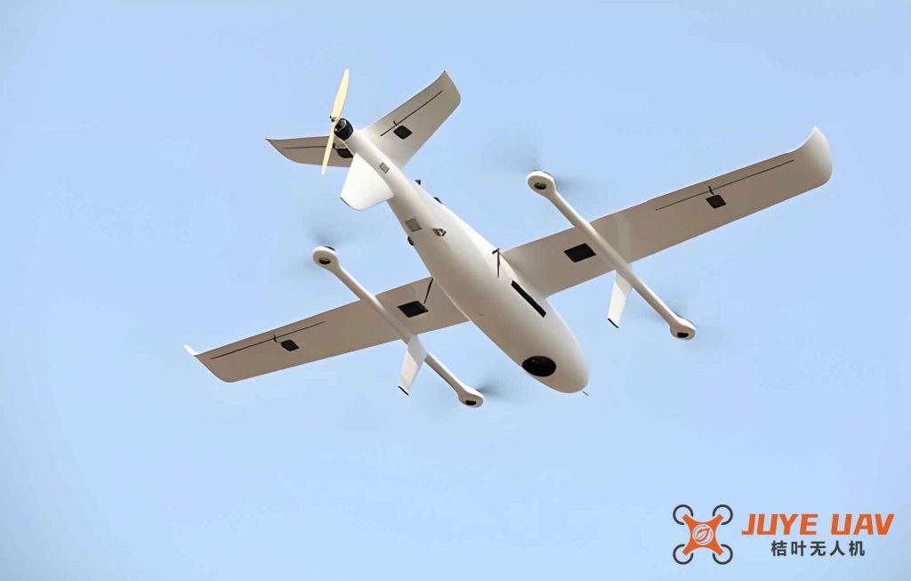
In our research, we address the challenge of cooperative patrol coverage path planning for fixed-wing drones operating in complex mountainous environments. Fixed-wing drones, with their high speed, low cost, and ability to carry sophisticated reconnaissance equipment, are increasingly deployed for persistent surveillance missions. Unlike previous works that focus on complete area coverage in a single pass, we emphasize continuous visitation of every point in the mission area through multi-drone coordination. Our approach enables drones to collaborate over the entire region rather than being assigned to isolated subareas, improving coverage efficiency and allowing flexible responses to emergency situations.
We model the mission space by discretizing the ground and flight volumes into grids. The ground grid size is finer than the flight grid to capture terrain details. Each ground cell maintains a state variable representing the time elapsed since its last visit. The flight grid cells are classified as safe (1), near-obstacle (0), or forbidden (-1) based on proximity to no-fly zones or obstacles. Fixed-wing drones move between flight grid centers, with four possible motion types due to the non-cubic grid geometry (horizontal and vertical dimensions differ). To ensure coordination, all drones adjust their velocities so that they reach the next waypoint simultaneously, eliminating temporal discrepancies.
The reconnaissance payload of a fixed-wing drone is mounted with a fixed downward angle. The field of view is determined by the pitch angle, heading angle, and limits: left/right angles \(\theta_{le}, \theta_{ri}\), front/back angles \(\theta_{fr}, \theta_{ba}\), and maximum sight range \(R\). The coverage area on the ground is computed by checking all candidate ground cells within a bounding box for three conditions: the cell’s four vertices lie inside the camera’s projected quadrilateral, within distance \(R\), and without any terrain occlusion. We derive the boundary of the search box for each of the eight cardinal headings as shown in Table 1.
| Heading | x-range | y-range |
|---|---|---|
| 0° | \([x_0, \min\{L_x, x_0 + R\sin(75°+\theta_{pit})\}]\) | \([\max\{0, y_0 + R\sin\theta_x\}, \min\{L_y, y_0 – R\sin\theta_x\}]\) |
| 45° | \([x_0, \min\{L_x, x_0 + R\sin(75°+\theta_{pit})\cos\theta_x\}]\) | \([y_0, \min\{L_y, y_0 + R\sin(75°+\theta_{pit})\sin\theta_x\}]\) |
| 90° | \([\max\{0, x_0 – R\cos\theta_x\}, \min\{L_x, x_0 + R\cos\theta_x\}]\) | \([y_0, \min\{L_y, y_0 + R\sin(75°+\theta_{pit})\}]\) |
| 135° | \([\max\{0, x_0 + R\sin(75°+\theta_{pit})\cos\theta_x\}, x_0]\) | \([y_0, \min\{L_y, y_0 + R\sin(75°+\theta_{pit})\sin\theta_x\}]\) |
| 180° | \([\max\{0, x_0 – R\sin(75°+\theta_{pit})\}, x_0]\) | \([\max\{0, y_0 – R\sin\theta_x\}, \min\{L_y, y_0 + R\sin\theta_x\}]\) |
| 225° | \([\max\{0, x_0 + R\sin(75°+\theta_{pit})\cos\theta_x\}, x_0]\) | \([\max\{0, y_0 – R\sin(75°+\theta_{pit})\sin\theta_x\}, y_0]\) |
| 270° | \([\max\{0, x_0 + R\cos\theta_x\}, \min\{L_x, x_0 – R\cos\theta_x\}]\) | \([\max\{0, y_0 – R\sin(75°+\theta_{pit})\}, y_0]\) |
| 315° | \([0, \min\{0, x_0 + R\sin(75°+\theta_{pit})\cos\theta_x\}]\) | \([\max\{0, y_0 + R\sin(75°+\theta_{pit})\sin\theta_x\}, y_0]\) |
To guide the drones toward areas that have not been visited for a long time, we define a state variable for each ground grid \(k\) at step \(s\):
$$sv_k(s) = 1 – \frac{t_v}{t_c(s)}$$
where \(t_v\) is the last time the grid was visited and \(t_c(s)\) is the current time. If the grid has never been visited, \(t_v = 0\) and \(sv_k(s)=1\). The overall surveillance metric for a drone at step \(s\) is the sum of state values over all covered grids:
$$J(s) = \sum_{m=1}^{g(s)} sv_m(s)$$
For grids that remain unvisited beyond a threshold \(\Delta T_v\), we introduce a weighted metric to attract the drone:
$$J(s) = g(s) \times \max\{sv_1(s), sv_2(s), \dots, sv_{g(s)}(s)\}$$
Multi-drone coordination is achieved through a sequential planning rule. All drones share a common matrix recording the visitation times of ground grids. After one drone completes its path planning, it updates the matrix for the next drone. To avoid multiple drones being attracted to the same high-value area, we adopt a simulated annealing approach to determine the planning order. For collision avoidance, we consider two types of conflicts: node collisions (two drones choosing the same waypoint at the same time) and path-crossing collisions (paths intersect between waypoints). The conditions are:
Node collision: \(\mathbf{p}_i(t+1) = \mathbf{p}_j(t+1)\)
Path-crossing collision: \(\mathbf{p}_i(t) + \mathbf{p}_i(t+1) = \mathbf{p}_j(t) + \mathbf{p}_j(t+1)\)
During planning, each drone avoids waypoints that would lead to either type of collision.
When an emergency arises—such as a target area that has been unvisited for too long or a sudden task requiring immediate full coverage—the system selects the nearest fixed-wing drone. This drone is assigned a higher priority and instructed to perform a two-phase mission: first, approach the emergency area while maintaining normal patrol efficiency using a dynamic target point strategy; second, conduct two rounds of shuttle coverage to achieve complete coverage.
In the approach phase, we set a distance threshold \(L_{max}\) derived from the centroid of the emergency area:
$$L_{max} = 2 \times \sqrt{(x_c – x_0)^2 + (y_c – y_0)^2 + (z_c – z_0)^2}$$
At each step, the drone checks candidate waypoints that satisfy the constraint:
$$L_{pre} + L_i + L_i^{tar} \leq L_{max}$$
where \(L_{pre}\) is the distance already traveled, \(L_i\) is the distance from the current node to candidate \(i\), and \(L_i^{tar}\) is the distance from candidate \(i\) to the current dynamic target (the nearest node to the emergency area). As the drone moves, the dynamic target point is updated step by step. Once the constraint fails or pathfinding fails, the drone switches to a standard A* algorithm to fly directly to the static target.
The standard A* algorithm is modified to incorporate the turning constraints of fixed-wing drones. For each candidate expansion, we check four conditions: (1) grid state not forbidden and not in the closed list; (2) satisfies the maximum turning angle constraint; (3) at least one subsequent move exists without immediate dead-end; (4) if adjacent to the goal, the entry direction must be compatible with the goal’s required exit direction. This ensures the generated path is flyable.
For the shuttle coverage phase, we first identify the cone-shaped airspace above each ground grid of the emergency area. To reduce computational complexity, the emergency area grids are coarsened to match the flight grid size. The coverage problem then becomes visiting all corresponding cones. In the first round, the drone travels from one cone to the nearest unvisited cone using the modified A* without directional constraints at the end, aiming to visit every cone once. After the first round, any uncovered grids are removed and their cones are deleted. In the second round, the drone re-enters the remaining cones with a directional constraint that forces the exit direction toward the cone’s axis, maximizing the probability of covering the ground cell. This two-round strategy guarantees complete coverage of the emergency area.
We conducted extensive simulations to validate the proposed algorithms. The mission space parameters are listed in Table 2.
| Parameter | Value |
|---|---|
| \(\theta_{fr}, \theta_{ba}, \theta_{le}, \theta_{ri}\) | 30° |
| Flight grid size (a, b, h) | 1000 m, 1000 m, 100 m |
| Mission area x, y, z limits | [0,50] km, [0,50] km, [0,5] km |
| Threshold \(\Delta T_v\) | 20 steps |
| Number of drones \(N_d\) | 5 (default), up to 10 |
| Ground grid size (ag, bg) | 100 m, 100 m |
| Full area \(L_x, L_y\) | 50 km, 50 km |
In the first set of experiments, five fixed-wing drones performed persistent surveillance without no-fly zones. Their trajectories converged to an altitude band of 3.0–3.8 km, where the field of view balanced terrain occlusion and resolution. The coverage heatmap showed that higher terrain (mountains and ridges) was visited more frequently than valleys, and boundary areas received slightly fewer visits due to a no-fly buffer. When random no-fly zones were introduced at the same altitude band, one zone directly blocked the optimal flight level. The drones detoured laterally without changing altitude, confirming that the preferred altitude offers significantly higher surveillance value than other layers. The state variable \(sv\) stabilized after about 800 steps, with the average value across grids decreasing smoothly. The algorithm demonstrated robust performance even with obstacles, though the area directly below the no-fly zone showed higher \(sv\) values due to avoidance.
To determine the optimal number of drones, we ran simulations with 3 to 10 fixed-wing drones. Figure 1 (not referenced) shows that increasing from 3 to 8 drones progressively reduced the average \(sv\) value and accelerated convergence. Beyond 8 drones, the improvement became marginal. For a 50 km × 50 km area, 8 drones provided the best trade-off between coverage efficiency and resource cost. Higher numbers led to redundant revisiting of recently visited areas.
In emergency scenarios, one drone (Drone 5) was tasked to cover a designated emergency area starting at step 200. Using the dynamic target point strategy, Drone 5 continued to contribute to overall surveillance while approaching the emergency zone. It reached the area in 29 steps (step 229) versus 20 steps (step 220) with a static target strategy. However, the average \(sv\) of the entire area showed significantly less degradation during the approach, indicating that the dynamic strategy better maintained normal patrol efficiency. After completing the two-round shuttle coverage, the emergency area was fully covered.
The efficiency comparison between static and dynamic target strategies for steps 200–235 is illustrated in the simulation data. The dynamic strategy kept the average \(sv\) lower (better) during the emergency response period, validating its superiority for missions where both responsiveness and continuous surveillance are critical. The shuttle coverage algorithm successfully achieved complete coverage of the emergency region by first scanning all cones and then specifically targeting any remaining uncovered cells.
We summarize the key contributions of our work:
- We formulated a patrol coverage path planning method for fixed-wing drones that continuously monitors entire areas with variable visitation intervals, using a state variable to quantify area importance.
- A multi-drone coordination mechanism based on sequential planning and local collision avoidance ensures safe and efficient sharing of the airspace.
- An emergency task handling approach with dynamic target points and a two-round shuttle coverage algorithm allows a fixed-wing drone to respond promptly while maintaining normal patrol duties.
- A modified A* algorithm with turning constraints and directional feasibility checks generates flyable paths for fixed-wing drones in complex 3D environments.
In conclusion, our cooperative path planning framework enables fixed-wing drones to execute persistent surveillance with high flexibility. The integration of dynamic target points and shuttle coverage makes it suitable for both routine monitoring and urgent ad-hoc tasks. Future work can extend the algorithm to more realistic scenarios including communication constraints, dynamic obstacles, and heterogeneous drone teams.