
In recent years, unmanned aerial vehicles (UAVs) have seen widespread adoption in both military and civilian domains. Among various types, the quadrotor drone stands out due to its simple structure, lightweight design, agility, and capabilities for vertical take-off, landing, and hovering. These attributes make the quadrotor drone a prominent platform for applications ranging from surveillance and delivery to environmental monitoring. However, the flight control system (FCS) of a quadrotor drone is critical for ensuring safe and reliable operation. Assessing the health and performance of the FCS often requires anomalous sensing data, which is typically scarce in real-world flight tests due to safety and cost constraints. This scarcity hinders the development and validation of anomaly detection methods, which are essential for predictive maintenance and fault prevention. To address this, I propose a method for generating anomalous attitude sensing data based on a physical simulation model of the quadrotor drone’s FCS. This approach leverages modeling and simulation techniques to create diverse anomalous datasets, enabling comprehensive evaluation of anomaly detection algorithms without risking actual hardware.
The core of my method involves developing a high-fidelity physical simulation model that replicates the dynamics and control logic of a quadrotor drone. By injecting anomalies into this model, I can generate realistic anomalous data for key attitude parameters, such as roll, pitch, and yaw angles and rates. This data can then be used to train and test anomaly detection models, such as those based on principal component analysis (PCA), to assess their effectiveness under various fault scenarios. In this article, I detail the modeling process, validation against real flight data, anomaly generation, and evaluation results. I emphasize the use of equations and tables to summarize key concepts and results, ensuring clarity and reproducibility. Throughout, the term ‘quadrotor drone’ is frequently used to maintain focus on the specific UAV type under study.
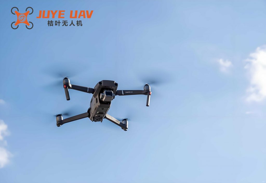
To begin, I define the coordinate systems essential for describing the motion of a quadrotor drone. Two primary coordinate frames are used: the ground-fixed frame \( S_g – O_g x_g y_g z_g \) and the body-fixed frame \( S_b – O x y z \). The ground frame has its origin at a point on the ground, with \( x_g \) pointing north, \( y_g \) pointing east, and \( z_g \) pointing downward toward the Earth’s center. The body frame is attached to the drone’s center of mass, with \( x \) pointing forward along the rotor arm, \( y \) pointing right, and \( z \) pointing downward. The orientation of the quadrotor drone is described by three Euler angles: roll (\( \phi \)), pitch (\( \theta \)), and yaw (\( \psi \)). The transformation matrix from the ground frame to the body frame, \( R_{g \to b} \), is given by:
$$ R_{g \to b} = \begin{bmatrix}
\cos\theta \cos\psi & \cos\theta \sin\psi & -\sin\theta \\
\sin\phi \sin\theta \cos\psi – \cos\phi \sin\psi & \sin\phi \sin\theta \sin\psi + \cos\phi \cos\psi & \sin\phi \cos\theta \\
\cos\phi \sin\theta \cos\psi + \sin\phi \sin\psi & \cos\phi \sin\theta \sin\psi – \sin\phi \cos\psi & \cos\phi \cos\theta
\end{bmatrix} $$
The inverse transformation, from body to ground frame, is \( R_{b \to g} = R_{g \to b}^T \). These transformations are crucial for converting forces and moments between frames when deriving the equations of motion.
Next, I establish the equations of motion for the quadrotor drone using Newton-Euler formulations. The drone is subject to gravitational forces and forces and moments generated by its four rotors. Each rotor produces a thrust \( F_i \) and a torque \( M_i \), which depend on the rotor’s angular speed \( \omega_i \):
$$ F_i = k_F \omega_i^2, \quad M_i = k_M \omega_i^2 $$
Here, \( k_F \) and \( k_M \) are thrust and torque coefficients, respectively. The total force and moment vectors in the body frame are derived from the geometry of the quadrotor drone. Let \( L \) be the distance from the center of mass to each rotor. The equations for linear and angular motion are:
Linear Motion (in ground frame):
$$ m \ddot{\mathbf{r}} = \begin{bmatrix} 0 \\ 0 \\ -mg \end{bmatrix} + R_{b \to g} \begin{bmatrix} 0 \\ 0 \\ \sum_{i=1}^4 F_i \end{bmatrix} $$
where \( m \) is the mass, \( \mathbf{r} = [x, y, z]^T \) is the position vector, and \( g \) is gravitational acceleration.
Angular Motion (in body frame):
$$ I \begin{bmatrix} \dot{p} \\ \dot{q} \\ \dot{r} \end{bmatrix} = \begin{bmatrix} L(F_2 – F_4) \\ L(F_3 – F_1) \\ M_1 – M_2 + M_3 – M_4 \end{bmatrix} – \begin{bmatrix} p \\ q \\ r \end{bmatrix} \times I \begin{bmatrix} p \\ q \\ r \end{bmatrix} $$
Here, \( I \) is the inertia matrix, and \( [p, q, r]^T \) are the angular velocities in the body frame. These equations form the basis for simulating the dynamics of the quadrotor drone.
To control the quadrotor drone, I design a hierarchical control loop consisting of an inner attitude control loop and an outer position control loop. The attitude controller regulates roll, pitch, and yaw angles by computing desired rotor speeds. For hover, the thrust from all rotors balances gravity: \( 4 k_F \omega_h^2 = mg \), where \( \omega_h \) is the hover speed. Deviations from hover are controlled using proportional-derivative (PD) laws. For example, the control input for roll is:
$$ \Delta\omega_\phi = k_{p,\phi} (\phi_{\text{des}} – \phi) + k_{d,\phi} (\dot{\phi}_{\text{des}} – \dot{\phi}) $$
Similar expressions apply for pitch and yaw. The desired rotor speeds \( \omega_i^{\text{des}} \) are then computed as a linear combination of these control inputs and the hover component. For a typical quadrotor drone with rotors arranged in an X-configuration, the mapping is:
$$ \begin{bmatrix} \omega_1^{\text{des}} \\ \omega_2^{\text{des}} \\ \omega_3^{\text{des}} \\ \omega_4^{\text{des}} \end{bmatrix} = \begin{bmatrix} 1 & 0 & 1 & -1 \\ 1 & 1 & 0 & 1 \\ 1 & 0 & -1 & -1 \\ 1 & -1 & 0 & 1 \end{bmatrix} \begin{bmatrix} \omega_h + \Delta\omega_F \\ \Delta\omega_\phi \\ \Delta\omega_\theta \\ \Delta\omega_\psi \end{bmatrix} $$
The outer position controller generates desired attitude angles from position errors. Using a PID controller, the desired accelerations \( \ddot{x}_{\text{des}}, \ddot{y}_{\text{des}}, \ddot{z}_{\text{des}} \) are computed. For horizontal motion, small-angle approximations yield:
$$ \phi_{\text{des}} = \frac{1}{g} (\ddot{x}_{\text{des}} \sin\psi_T – \ddot{y}_{\text{des}} \cos\psi_T), \quad \theta_{\text{des}} = \frac{1}{g} (\ddot{x}_{\text{des}} \cos\psi_T + \ddot{y}_{\text{des}} \sin\psi_T) $$
where \( \psi_T \) is the target yaw angle. For vertical motion, \( \Delta\omega_F = \frac{m}{8 k_F \omega_h} \ddot{z}_{\text{des}} \). This control structure ensures that the quadrotor drone can track desired trajectories while maintaining stability.
I implement the entire model in Simulink, a graphical environment for dynamic system simulation. The Simulink model includes blocks for the attitude controller, motor dynamics, body dynamics, and position controller. This allows for real-time simulation of the quadrotor drone’s flight under various conditions. To validate the model, I compare its outputs with real flight data from an actual quadrotor drone. The validation involves feeding the same position commands into both the simulation and the real drone, then comparing attitude and position responses. Correlation coefficients between simulated and real data are calculated; a coefficient above 0.8 indicates strong agreement. For instance, the yaw angle from simulation and real flight might show a correlation of 0.85, confirming the model’s fidelity. This step is crucial to ensure that the generated data is representative of a real quadrotor drone’s behavior.
Once validated, I use the model to generate anomalous attitude sensing data. Anomalies are injected into sensor outputs within the simulation to mimic common sensor faults, such as constant bias and drift. These anomalies are introduced during specific time intervals in the simulation. For a constant bias anomaly, a fixed offset is added to a sensor reading (e.g., yaw rate). For a drift anomaly, a time-varying offset that increases linearly is added. The injection process modifies the sensor data in the feedback loop, affecting the control system and producing realistic anomalous patterns in multiple parameters. This approach allows for the creation of diverse datasets with varying anomaly magnitudes and durations. Below, I summarize the anomaly types and their mathematical representations in a table.
| Anomaly Type | Mathematical Form | Description |
|---|---|---|
| Constant Bias | \( y_{\text{anom}}(t) = y_{\text{true}}(t) + B \) for \( t \in [t_0, t_1] \) | A fixed offset \( B \) added to the true sensor value. |
| Drift | \( y_{\text{anom}}(t) = y_{\text{true}}(t) + D \cdot (t – t_0) \) for \( t \in [t_0, t_1] \) | A linearly increasing offset with rate \( D \). |
To illustrate, I simulate a 100-second flight of the quadrotor drone. For the first 90 seconds, the drone follows a nominal trajectory. At \( t = 90 \) seconds, I inject a constant bias of \( B = 0.5 \, \text{rad/s} \) into the yaw rate sensor. The simulation outputs attitude data (e.g., yaw rate, roll rate, altitude) that now contains anomalies. Similarly, for drift anomalies, I inject a drift with \( D = 0.1 \, \text{rad/s}^2 \). The generated data captures not only the direct sensor error but also the propagated effects on other states due to closed-loop control. This richness makes the data valuable for testing anomaly detection methods that rely on multivariate correlations.
With anomalous data in hand, I evaluate the performance of an anomaly detection method based on principal component analysis (PCA). PCA is a statistical technique that reduces data dimensionality and identifies outliers by analyzing residuals. I train a PCA model on normal data (e.g., from 10–60 seconds of simulation) to establish a baseline. Then, I test it on data containing anomalies (e.g., from 70–100 seconds). The detection is based on the squared prediction error (SPE) statistic, \( Q \). A threshold \( Q_\alpha \) is set from the training data; if \( Q_{\text{new}} > Q_\alpha \) for a test sample, it is flagged as anomalous. I compute standard metrics: false positive rate (FPR), false negative rate (FNR), and accuracy (ACC). Below is a table summarizing detection results for different anomaly magnitudes.
| Anomaly Type | Magnitude | FNR | FPR | ACC |
|---|---|---|---|---|
| Constant Bias | 0.1 rad/s | 0.0340 | 0.7320 | 0.7333 |
| 0.2 rad/s | 0.0340 | 0.3300 | 0.8673 | |
| 0.3 rad/s | 0.0340 | 0.0960 | 0.9453 | |
| 0.4 rad/s | 0.0340 | 0.0480 | 0.9613 | |
| 0.5 rad/s | 0.0340 | 0.0280 | 0.9680 | |
| Drift | 0.03 rad/s² | 0.0320 | 0.7240 | 0.7373 |
| 0.06 rad/s² | 0.0320 | 0.4400 | 0.8320 | |
| 0.09 rad/s² | 0.0320 | 0.1940 | 0.9073 | |
| 0.12 rad/s² | 0.0320 | 0.0860 | 0.9500 | |
| 0.15 rad/s² | 0.0320 | 0.0540 | 0.9607 |
The results show that PCA detection performance improves as anomaly magnitude increases, with accuracy rising from around 73% to over 96%. However, for subtle anomalies (e.g., small bias or drift), the FPR remains high, indicating limitations of PCA in distinguishing weak anomalies from normal variations. This highlights the need for more advanced detection algorithms, which can be developed and tested using the generated data. The ability to produce data with controlled anomaly characteristics is a key advantage of my simulation-based approach for quadrotor drone health monitoring.
In conclusion, I have presented a comprehensive method for generating anomalous attitude sensing data for quadrotor drones via physical simulation. By developing a detailed model of the quadrotor drone’s flight control system, validating it against real data, and injecting anomalies, I can create realistic datasets that mimic sensor faults like constant bias and drift. These datasets enable rigorous evaluation of anomaly detection methods, as demonstrated with PCA. The approach addresses the critical challenge of data scarcity in UAV health management and provides a flexible framework for testing and improving detection algorithms. Future work could extend this method to other anomaly types, such as intermittent faults or complex multi-sensor failures, further enhancing the robustness of quadrotor drone operational safety. The integration of such simulation tools into the development lifecycle of quadrotor drones can significantly accelerate advances in autonomous system reliability and maintenance strategies.