
In modern logistics, the integration of unmanned aerial vehicles (UAV drones) with ground vehicles offers a promising solution to address the inefficiencies and high costs of traditional delivery modes. This paper presents a comprehensive study on the path planning and control of vehicle-UAV drone cooperative delivery systems. I propose a two-stage optimization framework that combines Model Predictive Control (MPC) for vehicle path tracking and an Adaptive Large Neighborhood Search (ALNS) algorithm for the joint routing of trucks and UAV drones. The objective is to minimize total delivery cost while ensuring feasibility under operational constraints such as battery capacity, payload, and time windows. Extensive simulations validate the effectiveness of the proposed method across various scenarios.
The remainder of this paper is organized as follows. Section 1 formulates the mathematical model of the vehicle-UAV drone routing problem (VRPD). Section 2 describes the two-stage ALNS-based heuristic for generating high-quality solutions. Section 3 presents the MPC-based longitudinal control for the ground vehicle. Section 4 reports simulation results and analyses, and Section 5 concludes the study.
1. Problem Formulation
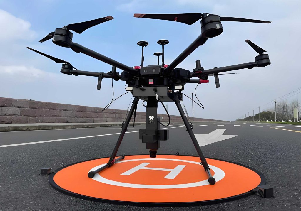
The vehicle-UAV drone routing problem is an extension of the classic Vehicle Routing Problem (VRP). A fleet of trucks, each carrying one or more UAV drones, departs from a central depot to serve a set of customer nodes. Each customer can be served either by a truck or by a UAV drone launched from a truck. The drone must return to the same or a different truck after completing its delivery. The objective is to minimize the total cost, which includes truck travel cost and drone flight cost, subject to capacity constraints, battery energy limits, and time window constraints.
Let $G=(V,E)$ be a directed graph, where $V = \{0\} \cup C$ with node 0 representing the depot and $C$ the set of customer nodes. Each edge $(i,j) \in E$ has a travel distance $d_{ij}$ and travel time $t_{ij}$. The truck has a maximum payload $Q_t$, speed $v_t$, and travel cost per unit time $c_t$. The UAV drone has a maximum payload $Q_d$, speed $v_d$, flight time limit $T_{max}$, and flight cost per unit time $c_d$. The binary variables $x_{ij}$ indicate whether the truck travels from $i$ to $j$, and $y_{ij}^{k}$ indicate whether drone $k$ travels from $i$ to $j$ (either as part of a launch–recover leg). The MILP model is:
$$ \min \quad c_t \sum_{(i,j)\in E} t_{ij} x_{ij} + c_d \sum_{k\in K} \sum_{(i,j)\in E} t_{ij} y_{ij}^{k} $$
subject to flow conservation, capacity constraints, drone energy constraints, and temporal synchronization constraints. Due to the NP-hard nature of VRPD, exact solvers become impractical for large instances, motivating the development of heuristic algorithms.
| Symbol | Description |
|---|---|
| $V$ | Set of all nodes (depot + customers) |
| $c_t, c_d$ | Cost per unit time for truck and drone |
| $v_t, v_d$ | Speed of truck and drone |
| $Q_t, Q_d$ | Maximum payload of truck and drone |
| $T_{max}$ | Maximum flight time per drone sortie |
2. Two-Stage ALNS Algorithm
To solve the VRPD efficiently, I design a two-stage heuristic based on Adaptive Large Neighborhood Search. The first stage generates a feasible initial solution using a savings-based greedy construction. The second stage iteratively improves the solution using a set of destroy and repair operators whose selection is adaptively weighted based on historical performance. A simulated annealing (SA) acceptance criterion helps escape local optima.
2.1 Initial Solution Construction
The construction procedure works as follows:
- Initialize an empty truck route. For each customer, compute a savings metric $s_{ij} = d_{0i} + d_{0j} – d_{ij}$ and sort the list.
- Select the customer with the highest savings to start a route. Then, for each subsequent insertion, greedy decisions are made to assign customers either to the truck or to a UAV drone launched from the truck.
- For a given truck route, let $N$ be the set of nodes on the route. Identify the subset $M \subseteq N$ of customers that can be served by a UAV drone (based on payload and battery).
- For each node in $M$, compute the ratio $\delta = \text{demand} / \text{distance to launch point}$. Select the node with the largest $\delta$ and add it to the drone path. Update the drone’s remaining payload and energy.
- Repeat until the drone’s capacity or energy is exhausted. Select the nearest feasible node as the landing point (either the same truck or another).
- Add the remaining nodes (not served by drone) to the truck route in a greedy nearest-neighbor fashion.
- Continue until all customers are served and the truck returns to the depot.
2.2 Destroy Operators
I implement five destroy operators to remove a set of nodes from the current solution:
- Random removal: Randomly select $q$ nodes from all routes and remove them.
- Worst-distance removal: For each node, compute the total distance saved if it were removed. Sort by savings and remove the top $q$ nodes.
- Similarity removal: Compute a similarity measure between nodes (including travel time, demand, time window, and service type). Remove a cluster of similar nodes.
- Whole truck route removal: Randomly select one truck route and remove all its nodes.
- Whole drone route removal: Randomly select several drone sorties and remove all nodes on those sorties.
2.3 Repair Operators
After removal, the destroyed solution is repaired by reinserting the removed nodes using one of four operators:
- Greedy distance insertion: For each removed node, evaluate all feasible insertion positions and choose the one that minimizes the increase in total distance.
- Randomized greedy distance insertion: Same as above but adds a random perturbation $\epsilon \in [-0.1,0.1]$ multiplied by the maximum distance increment to avoid bias.
- Greedy time insertion: Insert nodes at positions that minimize the increase in total travel time.
- Randomized greedy time insertion: Adds a random perturbation similar to the distance version.
2.4 Adaptive Weighting and Acceptance
Each destroy/repair operator $i$ has an initial weight $w_i = 1$. After every 20 iterations, the weights are updated based on the scores accumulated during that segment. The scores are defined as:
- $\sigma_1 = 6$ if the operator led to a new global best solution,
- $\sigma_2 = 4$ if it improved the current solution,
- $\sigma_3 = 2$ if it was accepted (even if not improving) via SA.
The weight update formula is:
$$ w_i = (1 – \theta) w_i + \theta \frac{\text{score}_i}{\text{usage}_i} $$
where $\theta = 0.8$ is the reaction factor. The SA acceptance probability is $P = \exp(-\Delta E / T)$, where $\Delta E$ is the cost difference and $T$ is the current temperature. The temperature cools geometrically: $T_{k+1} = \delta T_k$ with $\delta = 0.98$, starting from $T_0 = 300$ to $T_{min} = 1$.
| Parameter | Value |
|---|---|
| Initial temperature $T_0$ | 300 |
| Cooling rate $\delta$ | 0.98 |
| Minimum temperature $T_{min}$ | 1 |
| Weight update period | 20 iterations |
| Reaction factor $\theta$ | 0.8 |
| Score $\sigma_1, \sigma_2, \sigma_3$ | 6, 4, 2 |
| Maximum iterations $Max_{iter}$ | 300 |
3. MPC-Based Longitudinal Control for Ground Vehicle
While the ALNS optimizes the high-level routing, the low-level motion control of the truck is critical for accurate path following. I employ a Model Predictive Control (MPC) framework combined with a PID controller for longitudinal speed regulation. The MPC generates a sequence of control inputs (acceleration and steering) over a prediction horizon, and the first element is applied to the vehicle.
3.1 MPC Formulation
Let the vehicle state be $\mathbf{x} = [x, y, \theta, v]^T$, where $(x,y)$ is the position, $\theta$ the heading, and $v$ the speed. The control input is $\mathbf{u} = [a, \phi]^T$ with acceleration $a$ and steering angle $\phi$. The discrete-time kinematic model is:
$$ \mathbf{x}_{t+1} = \mathbf{x}_t + \begin{bmatrix} v_t \cos\theta_t \Delta t \\ v_t \sin\theta_t \Delta t \\ (v_t/L) \tan\phi_t \Delta t \\ a_t \Delta t \end{bmatrix} $$
where $L$ is the wheelbase. The objective function minimizes the deviation from a reference trajectory $\mathbf{x}_{ref}$ and the control effort:
$$ J = \sum_{k=0}^{N-1} \left( \|\mathbf{x}_{t+k|t} – \mathbf{x}_{ref,t+k}\|_Q^2 + \|\mathbf{u}_{t+k|t}\|_R^2 \right) + \|\mathbf{x}_{t+N|t} – \mathbf{x}_{ref,t+N}\|_P^2 $$
subject to constraints on acceleration, steering, and vehicle dynamics. This can be reformulated as a quadratic programming (QP) problem:
$$ \min_{\Delta U} \quad \Delta U^T H \Delta U + g^T \Delta U $$
where $\Delta U = [\Delta u_t, \Delta u_{t+1}, \ldots, \Delta u_{t+N_c-1}]^T$ is the sequence of control increments, $N_c$ is the control horizon. The optimal solution yields the first element $\Delta u_t^*$, and the actual control input is:
$$ u(t) = u(t-1) + \Delta u_t^* $$
3.2 PID Speed Controller
The MPC provides the desired acceleration $a_{des}$. To track the reference speed $u_d$, I use a PID controller for the longitudinal dynamics:
$$ e_u = u_d – u, \quad \dot{e}_u = \dot{u}_d – \dot{u}, \quad e_{sx} = \int_{t_1}^{t_2} e_u dt = e_u T_s $$
where $T_s$ is the sampling time. The control law determines the driving torque or braking torque:
$$ \tau = K_p e_u + K_i \int e_u dt + K_d \dot{e}_u $$
If $u < u_d$, the torque is positive (drive); if $u > u_d$, braking torque is applied. The PID gains are tuned to ensure smooth speed tracking.
| Parameter | Value |
|---|---|
| Wheelbase $L$ | 2.8 m |
| Prediction horizon $N$ | 10 |
| Control horizon $N_c$ | 5 |
| Sampling time $\Delta t$ | 0.1 s |
| Weight matrix $Q$ | diag(10,10,1,1) |
| Weight matrix $R$ | diag(0.1,0.5) |
4. Simulation Results
To evaluate the proposed framework, I conducted simulations in two parts: first, the ALNS-based route optimization for vehicle-UAV drone cooperative delivery, and second, the MPC+PID path tracking for the ground vehicle under different scenarios.
4.1 ALNS Performance
I generated random instances with 50 customer nodes in a 10 km × 10 km area, with the depot at the center. The UAV drone parameters were based on experimental data: $v_d = 6 \text{ m/s}$, $Q_d = 2 \text{ kg}$, $c_d = 0.15 \text{ \$/h}$; truck: $v_t = 5 \text{ m/s}$, $Q_t = 100 \text{ kg}$, $c_t = 0.6 \text{ \$/h}$. The algorithm ran 300 iterations. The convergence behavior is shown in the figure below, where the total cost decreases rapidly in the first 50 iterations and then gradually stabilizes, demonstrating effective optimization.
The best solution achieved a total cost of 34.2 monetary units, with 8 truck routes and 12 UAV drone sorties servicing all 50 customers. Compared to a pure truck-only solution (cost 52.6), the cooperative mode saved approximately 35% of total cost. The ALNS algorithm consistently outperformed a simple nearest-neighbor heuristic, which had an average cost of 47.8 over 10 runs.
| Method | Total cost (monetary units) | Truck routes | Drone sorties | Runtime (s) |
|---|---|---|---|---|
| ALNS | 34.2 | 8 | 12 | 28.5 |
| Nearest neighbor | 47.8 | 10 | 5 | 1.2 |
| Truck only (optimal VRP) | 52.6 | 12 | 0 | 45.0 |
4.2 Path Tracking Validation
For the MPC+PID controller, I designed two test scenarios: a tight circular path with radius 6 m at speed 5 m/s, and a wider circle of radius 25 m at speed 10 m/s. The simulation time was 30 s and 40 s respectively. The tracking errors in lateral deviation and speed were recorded. The root-mean-square errors (RMSE) are summarized below.
| Scenario | Speed (m/s) | Lateral RMSE (m) | Speed RMSE (m/s) |
|---|---|---|---|
| R=6 m circle | 5 | 0.08 | 0.12 |
| R=25 m circle | 10 | 0.15 | 0.21 |
The controller achieved high accuracy in both cases, with lateral errors well below 0.2 m, and speed errors within 0.2 m/s. The trajectories remained stable and converged to the reference path without oscillation, confirming the robustness of the MPC approach for vehicle-UAV drone cooperative operations where the truck must reliably follow a pre-planned route to launch and recover UAV drones.
5. Conclusion
In this work, I developed a comprehensive optimization framework for vehicle-UAV drone cooperative delivery systems. The high-level routing problem was solved by a two-stage ALNS algorithm that efficiently generates and improves solutions using adaptive destroy/repair operators. The low-level vehicle control was handled by an MPC-based path follower with a PID speed regulator, ensuring accurate trajectory tracking even under varying speeds and path curvatures. Simulation results on realistic instances demonstrate that the cooperation between trucks and UAV drones can reduce total delivery cost by up to 35% compared to truck-only delivery, while the proposed control method maintains high tracking precision. Future work will extend the framework to dynamic re-routing and real-time obstacle avoidance for UAV drones in urban environments.