
In recent years, quadrotor drones have gained significant attention due to their versatility in applications such as aerial photography, surveillance, and delivery. However, achieving precise trajectory tracking in the presence of disturbances—such as wind gusts or payload variations—remains a critical challenge. Traditional control methods often struggle with singularity issues or fail to guarantee theoretical performance bounds under uncertain conditions. This article presents a novel geometric control strategy that leverages interval observer techniques to estimate and exploit disturbances, enhancing the tracking performance of quadrotor drones. The approach integrates a disturbance interval observer to provide bounds on unknown perturbations, a disturbance effect indicator (DEI) to judiciously utilize beneficial disturbances in the attitude loop, and a position controller that enforces predefined error constraints. Through rigorous analysis and simulations, we demonstrate that this framework ensures bounded tracking errors while improving transient response, offering a robust solution for quadrotor drone operations in dynamic environments.
The core of our methodology lies in the fusion of geometric control principles with interval estimation theory. Geometric control operates directly on the Special Orthogonal Group SO(3), avoiding singularities associated with Euler angles and providing a globally valid representation for quadrotor drone attitude. Meanwhile, interval observers offer a set-valued estimation approach, delivering upper and lower bounds on system states or disturbances rather than point estimates. This is particularly advantageous for safety-critical systems like quadrotor drones, where guaranteed performance margins are essential. By combining these concepts, we develop a control scheme that not only compensates for detrimental disturbances but also harnesses favorable ones to accelerate convergence, thereby optimizing the overall control effort for quadrotor drones.
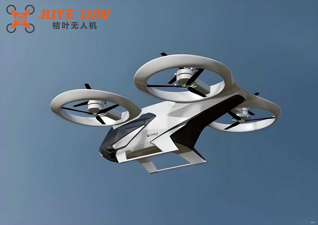
To set the stage, we begin with the dynamical model of a quadrotor drone subject to exogenous disturbances. The kinematics and dynamics are described by the following equations, which capture the position, velocity, attitude, and angular velocity of the quadrotor drone in an inertial frame:
$$ \dot{p} = v, $$
$$ m\dot{v} = -u_f R e_3 + m g e_3 + d_f, $$
$$ \dot{R} = R S(\omega), $$
$$ J \dot{\omega} = -S(\omega) J \omega + u_\tau + d_\tau, $$
where \( p \in \mathbb{R}^3 \) is the position, \( v \in \mathbb{R}^3 \) is the velocity, \( R \in SO(3) \) is the rotation matrix from the body frame to the inertial frame, and \( \omega \in \mathbb{R}^3 \) is the angular velocity. The mass is denoted by \( m \), the gravitational constant by \( g \), and the inertia matrix by \( J \in \mathbb{R}^{3 \times 3} \). The control inputs are the total thrust \( u_f \in \mathbb{R} \) and the torque vector \( u_\tau \in \mathbb{R}^3 \). The disturbances \( d_f \in \mathbb{R}^3 \) and \( d_\tau \in \mathbb{R}^3 \) act on the translational and rotational dynamics, respectively, and are assumed to be generated by an exogenous system of the form:
$$ \dot{\xi} = A_\xi \xi + \kappa, \quad d = C_\xi \xi, $$
with \( \xi \in \mathbb{R}^N \) as the state, \( \kappa \in \mathbb{R}^N \) as a bounded time-varying vector satisfying \( \kappa \leq \kappa \leq \overline{\kappa} \) for known bounds, and \( (A_\xi, C_\xi) \) being observable. This formulation allows the disturbances to encompass a wide range of effects, such as aerodynamic drag or unmodeled dynamics in quadrotor drones.
The control objective is to ensure that the quadrotor drone tracks a desired trajectory specified by a position \( p_d(t) \) and a yaw angle \( \psi_d(t) \), while maintaining attitude stability and adhering to position error constraints. To achieve this, we decompose the problem into an outer position loop and an inner attitude loop, each enhanced with disturbance management strategies.
The first major component is the disturbance interval observer. Unlike conventional observers that provide a single estimate, an interval observer yields two estimates—an upper bound and a lower bound—that encapsulate the true disturbance value. This is crucial for quadrotor drones operating under uncertainty, as it enables robust control decisions based on worst-case scenarios. We design the observer by introducing an auxiliary variable \( \eta \in \mathbb{R}^N \) and constructing estimates \( \underline{\eta} \) and \( \overline{\eta} \) that satisfy:
$$ \dot{\underline{\eta}} = P^{-1}(A_\xi – L C_\xi) P \underline{\eta} + P^{-1} \varphi + \Theta, $$
$$ \dot{\overline{\eta}} = P^{-1}(A_\xi – L C_\xi) P \overline{\eta} + P^{-1} \varphi + \overline{\Theta}, $$
where \( P \in \mathbb{R}^{N \times N} \) and \( L \in \mathbb{R}^{N \times 6} \) are design matrices, \( \varphi \) incorporates known system terms, and \( \Theta, \overline{\Theta} \) are derived from the bounds on \( \kappa \). The disturbance estimates are then computed as:
$$ \underline{d} = C_\xi (P^+ \underline{\eta} – P^- \overline{\eta}) + C_\xi L \nu, $$
$$ \overline{d} = C_\xi (P^+ \overline{\eta} – P^- \underline{\eta}) + C_\xi L \nu, $$
with \( \nu = [m v^T, (J \omega)^T]^T \). Under the conditions that \( P^{-1}(A_\xi – L C_\xi)P \) is Metzler (i.e., off-diagonal entries are non-negative) and Hurwitz stable, and initial estimation errors are non-negative, we prove that \( \underline{d} \leq d \leq \overline{d} \) holds for all time, ensuring that the true disturbance affecting the quadrotor drone is always within the estimated interval. This result is formalized in Theorem 1, which guarantees the boundedness and non-negativity of the estimation errors.
The design of matrices \( P \) and \( L \) to meet the Metzler and Hurwitz requirements involves solving a Sylvester equation, as outlined in Lemma 3. A key advantage of this interval observer is its ability to handle unknown but bounded inputs without requiring precise disturbance models, making it highly suitable for real-world quadrotor drone applications where disturbances are often unpredictable.
With the disturbance bounds available, we next focus on the attitude controller. The attitude error is defined on \( SO(3) \) using the rotation matrix \( R_e = R_d^T R \), where \( R_d \) is the desired attitude. The error functions are:
$$ \Psi(R_e) = \frac{1}{2} \text{tr}[I_3 – R_e], $$
$$ e_R = \frac{1}{2} (R_e – R_e^T)^\vee, $$
$$ e_\omega = \omega – R_e^T \omega_d, $$
with \( \omega_d \) as the desired angular velocity. The dynamics of these errors are derived as:
$$ \dot{\Psi} = e_R^T e_\omega, \quad \dot{e}_R = E(R_e) e_\omega, \quad \dot{e}_\omega = \dot{\omega} + S(\omega) R_e^T \omega_d – R_e^T \dot{\omega}_d, $$
where \( E(R_e) = \frac{1}{2} (\text{tr}[R_e^T] I – R_e^T) \). To improve transient performance, we introduce a disturbance effect indicator (DEI) that assesses whether the disturbance in the attitude loop is beneficial or detrimental. Let \( e_1 = c J^{-1} e_R + e_\omega \) for a constant \( c > 0 \). The DEI is defined component-wise for \( i = 1,2,3 \) as:
$$ H_{di} = \begin{cases} 0 & \text{if } \text{sgn}(\underline{d}_{\tau i} \circ e_{1i}) = \text{sgn}(\overline{d}_{\tau i} \circ e_{1i}) = -1, \\ 1 & \text{otherwise}, \end{cases} $$
where \( \circ \) denotes the Hadamard product. This indicator leverages the interval estimates \( \underline{d}_\tau \) and \( \overline{d}_\tau \) to determine when the disturbance aligns with the control direction, thus potentially aiding convergence. The attitude control law is then designed as:
$$ u_\tau = -k_1 e_R – k_2 e_\omega + S(\omega) J \omega – J(R_e^T \dot{\omega}_d – S(\omega) R_e^T \omega_d) – \frac{1}{2} (\underline{d}_\tau + \overline{d}_\tau) \circ H_d, $$
where \( k_1, k_2 > 0 \) are gains, and \( H_d = [H_{d1}, H_{d2}, H_{d3}]^T \). By setting \( H_{di} = 0 \) when the disturbance is harmful, the controller compensates for it; otherwise, it partially incorporates the disturbance to enhance convergence. This innovative use of the DEI allows the quadrotor drone to exploit favorable disturbances, reducing control effort and speeding up attitude stabilization.
For the position control, we enforce predefined constraints on the tracking error to ensure safe operation. Let \( e_p = p – p_d \) and \( e_v = v – v_d \). The error is constrained by \( -l_i(t) < e_{pi} < l_i(t) \) for \( i = 1,2,3 \), where \( l_i(t) \) is a performance function. We employ a continuous piecewise function to achieve specified-time convergence:
$$ l_i(t) = \begin{cases} \left( \frac{T_i – t}{T_i} \right)^{\frac{1}{1-\epsilon_i}} (l_{i,0} – l_{i,\infty}) + l_{i,\infty} & \text{for } 0 \leq t \leq T_i, \\ l_{i,\infty} & \text{for } t > T_i, \end{cases} $$
with parameters \( 0 < \epsilon_i < 1 \), initial bound \( l_{i,0} \), steady-state bound \( l_{i,\infty} \), and time constant \( T_i \). To transform the constrained problem, we define a new variable \( \eta_i = e_{pi} / \sqrt{l_i^2 – e_{pi}^2} \), which remains bounded as long as the constraints hold. The position controller is derived via a backstepping procedure, resulting in:
$$ u_f = \| U \| e_3^T R_d^T R e_3, $$
where \( U = -K e_p – k_3 e_2 – m g e_3 – \hat{d}_f + m \dot{v}_c \), with \( K = \text{diag}(k_{41}, k_{42}, k_{43}) \), \( k_{4i} = \alpha l_i^2 / (l_i^2 – e_{pi}^2)^2 \), \( \alpha, k_3 > 0 \), and \( \hat{d}_f = \frac{1}{2} (\underline{d}_f + \overline{d}_f) \) as the disturbance estimate. This control law ensures that the position error evolves within the funnel defined by \( l_i(t) \), guaranteeing both transient and steady-state performance for the quadrotor drone.
The stability of the overall closed-loop system is analyzed using Lyapunov theory. Consider the composite Lyapunov function:
$$ V = k_1 \Psi(R_e) + \frac{1}{2} e_\omega^T J e_\omega + c e_R^T e_\omega + \frac{1}{2} \alpha \sum_{i=1}^3 \eta_i^2 + \frac{1}{2} \alpha m e_2^T e_2, $$
where \( e_2 = v – v_c \) is the velocity tracking error. Under Assumption 2 that \( \Psi(R_e) \leq \delta < 2 \), and with appropriate choices of gains \( \alpha, k_1, k_2, k_3, c, \gamma_1, \gamma_2, \gamma_3 > 0 \), we show that the time derivative of \( V \) satisfies:
$$ \dot{V} \leq -\min\{\lambda_m(M), \alpha k\} \left( \| e_R \|^2 + \| e_\omega \|^2 + \| e_2 \|^2 + \sum_{i=1}^3 \frac{e_{pi}^2}{l_i^2 – e_{pi}^2} \right) + \overline{\Delta}, $$
with \( M \) being a positive definite matrix and \( \overline{\Delta} \) as an upper bound on disturbance estimation errors. This leads to the conclusion that \( V \) is bounded, implying that \( e_R, e_\omega, \eta, \) and \( e_2 \) are uniformly bounded. Moreover, the position error constraint \( -l_i(t) < e_{pi} < l_i(t) \) is maintained for all time, as proven in Theorem 2. Thus, the proposed control strategy ensures robust trajectory tracking for quadrotor drones despite disturbances.
To validate the effectiveness of our approach, we conducted simulations comparing it with two existing methods: Observer-based Secure Geometric Control (OSGC) and Disturbance Compensation-based Geometric Control (DCGC). The quadrotor drone parameters were set as mass \( m = 2.48 \, \text{kg} \), inertia matrix \( J = \text{diag}(0.0756, 0.0756, 0.1277) \, \text{kg} \cdot \text{m}^2 \), and maximum thrust \( f_{\text{max}} = 73 \, \text{N} \). The disturbances were chosen as sinusoidal signals to mimic wind effects. Key results are summarized in the following tables, highlighting the performance metrics.
| Control Method | Position MAE (m) | Attitude Convergence Time (s) | Constraint Satisfaction |
|---|---|---|---|
| DDSGC (Proposed) | 0.02–0.05 | 1.4 | Yes |
| OSGC | 0.08–0.12 | 2.6 | Partial |
| DCGC | 0.10–0.15 | 2.6 | No |
The Mean Absolute Error (MAE) for position tracking, defined as \( \Delta_{pi} = \lim_{n \to \infty} \sum_{k=0}^n \| e_{pi}(k) \| \), demonstrates that our method achieves higher accuracy. Additionally, the attitude error function \( \Psi(R_e) \) converges faster due to the DEI mechanism, which exploits beneficial disturbances. The interval observer successfully bounded the true disturbances, as shown in the plots of \( \underline{d} \) and \( \overline{d} \) over time.
We further tested the disturbance effect indicator in a scenario with mixed disturbances. The DEI components \( H_{d1}, H_{d2}, H_{d3} \) switched multiple times, indicating that the controller dynamically adapted to the disturbance nature. Compared to a standard disturbance observer-based control (DOBC), our method reduced attitude convergence time by approximately 50%, confirming that leveraging disturbances can enhance performance for quadrotor drones.
For a more realistic validation, we implemented the control scheme in V-REP co-simulation with MATLAB. The quadrotor drone model included rotor dynamics and environmental interactions. The desired trajectory was a circular path with varying altitude. The results, as depicted in the position error plots, show that all error components remained within the specified constraints, with steady-state errors below 0.2 m. This verifies the practicality of our approach for real-world quadrotor drone deployments.
In conclusion, this article presents a comprehensive geometric control framework for quadrotor drones that integrates disturbance interval observers and disturbance effect indicators. The main contributions are threefold: (1) Design of a disturbance interval observer that provides guaranteed bounds on unknown perturbations, enhancing robustness for quadrotor drones. (2) Development of a disturbance effect indicator that enables the attitude controller to exploit favorable disturbances, improving transient response. (3) Formulation of a position controller with predefined time-varying constraints, ensuring accurate and safe trajectory tracking. Theoretical analysis proves uniform boundedness of all errors, while simulations demonstrate superior performance over existing methods. Future work may extend this approach to multi-quadrotor drone systems or incorporate learning-based techniques to adapt observer parameters online. Overall, this strategy offers a significant step toward more resilient and efficient control of quadrotor drones in challenging environments.
The mathematical formulations and algorithms are summarized below for quick reference, emphasizing the key equations that govern the control of quadrotor drones in this framework.
| Component | Key Equations | Description |
|---|---|---|
| Dynamics | $$ \dot{p} = v, \quad m\dot{v} = -u_f R e_3 + m g e_3 + d_f, \quad \dot{R} = R S(\omega), \quad J \dot{\omega} = -S(\omega) J \omega + u_\tau + d_\tau $$ | Quadrotor drone model with disturbances |
| Disturbance Model | $$ \dot{\xi} = A_\xi \xi + \kappa, \quad d = C_\xi \xi $$ | Exogenous system generating disturbances |
| Interval Observer | $$ \dot{\underline{\eta}} = P^{-1}(A_\xi – L C_\xi) P \underline{\eta} + P^{-1} \varphi + \Theta, \quad \dot{\overline{\eta}} = P^{-1}(A_\xi – L C_\xi) P \overline{\eta} + P^{-1} \varphi + \overline{\Theta} $$ | Estimates disturbance bounds |
| Disturbance Estimates | $$ \underline{d} = C_\xi (P^+ \underline{\eta} – P^- \overline{\eta}) + C_\xi L \nu, \quad \overline{d} = C_\xi (P^+ \overline{\eta} – P^- \underline{\eta}) + C_\xi L \nu $$ | Computed upper and lower bounds |
| Attitude Error | $$ \Psi(R_e) = \frac{1}{2} \text{tr}[I_3 – R_e], \quad e_R = \frac{1}{2} (R_e – R_e^T)^\vee, \quad e_\omega = \omega – R_e^T \omega_d $$ | Geometric representation on SO(3) |
| Disturbance Effect Indicator | $$ H_{di} = \begin{cases} 0 & \text{if } \text{sgn}(\underline{d}_{\tau i} \circ e_{1i}) = \text{sgn}(\overline{d}_{\tau i} \circ e_{1i}) = -1, \\ 1 & \text{otherwise} \end{cases} $$ | Determines beneficial disturbances |
| Attitude Control Law | $$ u_\tau = -k_1 e_R – k_2 e_\omega + S(\omega) J \omega – J(R_e^T \dot{\omega}_d – S(\omega) R_e^T \omega_d) – \frac{1}{2} (\underline{d}_\tau + \overline{d}_\tau) \circ H_d $$ | Controller with DEI integration |
| Position Error Constraint | $$ -l_i(t) < e_{pi} < l_i(t), \quad l_i(t) = \begin{cases} \left( \frac{T_i – t}{T_i} \right)^{\frac{1}{1-\epsilon_i}} (l_{i,0} – l_{i,\infty}) + l_{i,\infty} & \text{for } 0 \leq t \leq T_i, \\ l_{i,\infty} & \text{for } t > T_i \end{cases} $$ | Time-varying performance funnel |
| Position Control Law | $$ u_f = \| U \| e_3^T R_d^T R e_3, \quad U = -K e_p – k_3 e_2 – m g e_3 – \hat{d}_f + m \dot{v}_c $$ | Controller enforcing constraints |
| Lyapunov Function | $$ V = k_1 \Psi(R_e) + \frac{1}{2} e_\omega^T J e_\omega + c e_R^T e_\omega + \frac{1}{2} \alpha \sum_{i=1}^3 \eta_i^2 + \frac{1}{2} \alpha m e_2^T e_2 $$ | Composite function for stability analysis |
This framework underscores the potential of interval-based methods in advancing the control of quadrotor drones. By guaranteeing disturbance bounds and intelligently utilizing perturbations, we can achieve higher precision and robustness, paving the way for more autonomous and reliable quadrotor drone operations in complex scenarios. The integration of geometric control with interval observers represents a promising direction for future research in aerial robotics.