
1. Introduction and Research Context
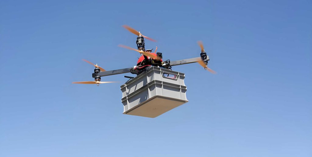
The rapid advancement of low-altitude economy and the continuous iteration of drone technology have propelled unmanned aerial vehicles (UAVs) from professional domains into mainstream applications, establishing them as indispensable tools for acquiring spatial information. Leveraging advantages such as operational flexibility, low cost, and extensive coverage, UAVs play irreplaceable roles in numerous fields including agricultural monitoring, power line inspection, environmental surveillance, emergency rescue, urban planning, and military reconnaissance. The global civilian UAV market has sustained double-digit growth for multiple consecutive years, with a market size exceeding 40 billion USD in 2023 and projected to reach 80 billion USD by 2028. Simultaneously, the volume of aerial imagery data generated has grown exponentially, forming vast spatial information resources. The detection of objects, particularly small objects, in imagery captured by unmanned aerial vehicles has emerged as a critical bottleneck constraining intelligent analysis and application of aerial data.
Compared with conventional ground-level photography, imagery acquired from unmanned aerial vehicles exhibits distinctive characteristics. First, the high-altitude top-down perspective significantly alters the morphological appearance, texture, and illumination conditions of objects, compressing the observable features of targets and rendering them difficult to identify. Second, the majority of objects of interest, such as pedestrians, vehicles, and small facilities, occupy extremely low pixel proportions, typically ranging from a few to tens of pixels, which severely limits the availability of discriminative details. Third, aerial scenes encompass complex and varied backgrounds, including urban structures, natural terrain, and vegetation, where objects are frequently subject to occlusion and blending with their surroundings. Fourth, while ensuring wide coverage, UAV imagery often suffers from ultra-high resolution accompanied by motion blur, illumination variation, and atmospheric scattering, all of which interfere with the stability of object features.
The technical evolution of object detection has undergone a paradigm shift from traditional hand-crafted feature extraction to deep learning-driven approaches. Traditional algorithms, such as HOG+SVM and DPM, rely on manually designed feature extractors, which offer limited representation capability for small objects and exhibit low detection accuracy and poor robustness in complex aerial scenes. In recent years, deep learning-based detection algorithms, including the YOLO series and Faster R-CNN, have achieved breakthrough progress in natural image detection tasks through powerful feature learning capabilities. However, these algorithms are primarily designed for conventionally sized objects in ground-level images, and their direct application to small object detection in UAV aerial imagery presents notable adaptation challenges. The shallow features of deep models struggle to capture effective information from small objects, while deep features tend to lose spatial details essential for accurate localization. Moreover, existing anchor design, positive-negative sample assignment strategies, and loss functions do not adequately account for the scale characteristics of small objects, resulting in generally low recall and precision. Research indicates that mainstream algorithms achieving above 90% accuracy on conventional images often see accuracy decline to below 50% when applied to small object detection in aerial imagery captured by unmanned aerial vehicles.
The core challenges in UAV aerial small object detection can be attributed to several factors: significant scale variation, sparse and easily obscured features of small objects, class imbalance, complex backgrounds, and computational constraints of onboard platforms. The unique perspective introduces domain shift issues when transferring ground-view pretrained models. These challenges underscore the pressing need for targeted algorithm research and technical innovation. This dissertation addresses these issues by proposing enhanced detection algorithms built upon the YOLOv11 framework, focusing on both high-precision detection and lightweight deployment for resource-constrained platforms.
2. Fundamentals of Object Detection in UAV Imagery
2.1 Convolutional Neural Networks
Convolutional Neural Networks (CNNs) constitute the foundational architecture for modern deep learning-based object detection systems. A typical CNN consists of convolutional layers, activation layers, pooling layers, and fully connected layers. The convolutional layer performs feature extraction through learnable kernels that slide over input feature maps, computing weighted sums over local receptive fields. Key parameters include kernel size, stride, padding, and the number of output channels. The stride determines the step size of kernel movement, directly controlling the spatial dimensions of output feature maps. Padding preserves edge information and controls output size. The number of output channels corresponds to the number of distinct feature detectors learned by the layer.
Activation layers introduce nonlinearity into the network, enabling the modeling of complex feature relationships. Several activation functions are widely employed: the Sigmoid function, defined as \(\sigma(x) = 1/(1+e^{-x})\), maps inputs to the range (0,1) but suffers from gradient vanishing; the Tanh function, \((\tanh(x) = (e^{x}-e^{-x})/(e^{x}+e^{-x}))\), is zero-centered and mitigates vanishing gradients but still saturates; the Rectified Linear Unit (ReLU), \(\text{ReLU}(x) = \max(0,x)\), alleviates gradient vanishing in the positive domain but can cause dead neurons; and the SiLU function, \(\text{SiLU}(x) = x \cdot \sigma(x)\), combines smoothness with nonlinear expressiveness. Pooling layers perform downsampling through operations such as max pooling, which retains the most salient features, or average pooling, which preserves background information. Fully connected layers integrate global features and map them to task-specific outputs, though they introduce substantial parameters and are increasingly replaced by global average pooling in modern architectures.
2.2 Deep Learning Detection Frameworks
Two predominant paradigms exist for deep learning-based object detection: two-stage and one-stage approaches. Two-stage detectors, exemplified by the R-CNN family, first generate region proposals and then perform classification and regression on these proposals. The Faster R-CNN architecture introduced the Region Proposal Network (RPN), which shares convolutional features with the detection network, enabling end-to-end training and achieving a balance between accuracy and efficiency. RPN generates region proposals by predicting objectness scores and bounding box regressions for a set of predefined anchors at multiple scales and aspect ratios. Despite their high accuracy, two-stage detectors often fall short of real-time requirements due to their complex cascaded structure.
One-stage detectors, such as the SSD, RetinaNet, and YOLO families, treat detection as a direct regression problem, predicting class probabilities and bounding box coordinates from feature maps in a single forward pass. The YOLO series has evolved through multiple generations, each contributing architectural refinements. YOLOv5 introduced adaptive anchor generation and mosaic data augmentation. YOLOv8 adopted a C2f module with richer gradient flow and an anchor-free decoupled head. The latest YOLOv11 incorporates the C3k2 module with dual-branch parallel convolution and multi-scale kernels, the C2PSA attention module for dynamic feature focusing, and an optimized lightweight decoupled detection head. These advancements have progressively improved the balance between detection accuracy, inference speed, and model compactness.
2.3 Datasets for UAV Aerial Detection
This research employs two widely recognized public datasets for unmanned aerial vehicles imagery. The VisDrone2019 dataset, developed by the AISKYEYE team at Tianjin University, contains 10,209 static images and 288 video clips captured across 14 different cities, covering altitudes from 20 to 120 meters and various lighting and weather conditions. The dataset provides approximately 2.6 million manually annotated bounding boxes covering ten common traffic categories including pedestrian, bicycle, car, van, truck, bus, tricycle, awning-tricycle, and motor. Table 1 presents the distribution of object sizes within the VisDrone2019 dataset. Objects smaller than 16×16 pixels constitute 12.05%, those between 16×16 and 32×32 pixels account for 32.65%, and objects larger than 32×32 pixels represent 55.30%. This distribution highlights the prevalence of small objects, which poses significant challenges for detection algorithms.
| Object Category (VisDrone2019) | Percentage of Objects <16×16 px | Percentage 16×16–32×32 px | Percentage >32×32 px |
|---|---|---|---|
| All categories | 12.05% | 32.65% | 55.30% |
The second dataset, DOTAv1.0, is a large-scale remote sensing benchmark containing 2,806 high-resolution images with 188,282 oriented bounding box annotations across 15 categories. The dataset covers diverse scenes including cities, harbors, airports, and agricultural areas, with ground resolutions ranging from 0.5 to 2.0 meters. The images exhibit arbitrary object orientations, extreme scale variations, and dense arrangements, providing a rigorous benchmark for evaluating the robustness and generalization capacity of detection algorithms.
2.4 Evaluation Metrics
The evaluation of detection algorithms employs several standard metrics. Precision (P) measures the proportion of correctly predicted positive samples among all predicted positive samples, \(P = TP/(TP+FP)\). Recall (R) measures the proportion of correctly detected positive samples among all actual positive samples, \(R = TP/(TP+FN)\). Here, TP denotes true positives, FP false positives, and FN false negatives. Average Precision (AP) summarizes the Precision-Recall curve for a single class, while mean Average Precision (mAP) averages AP across all classes. The metric mAP@0.5 refers to the mean AP computed at an IoU threshold of 0.5, while mAP@0.5:0.95 averages AP values across IoU thresholds ranging from 0.5 to 0.95 in increments of 0.05. Model complexity is assessed through the number of parameters (Params) and floating-point operations (GFLOPs), while inference speed is measured in frames per second (FPS).
3. PE-YOLO: High-Precision Detection Algorithm
3.1 Motivation and Overview
To address the challenges of insufficient feature extraction and limited localization accuracy for small objects in imagery from unmanned aerial vehicles, I propose a high-precision detection algorithm named PE-YOLO (Pixel Enhanced-YOLO), built upon the YOLOv11 baseline. The algorithm introduces four key innovations: the Multi-Dimensional Pixel Enhancement attention module (MDPE) in the backbone, the Dynamic Adaptive Feature Integration module (DAFI) in the neck, the Feature Alignment Dynamic Head (FADH) for detection, and the ARSIoU loss function for optimized regression. The overall architecture integrates these components to enhance feature extraction, fusion, and localization for small object detection in complex aerial scenes.
3.2 Multi-Dimensional Pixel Enhancement Attention Module (MDPE)
Small objects in imagery captured by unmanned aerial vehicles occupy extremely limited pixel regions, and their salient features are often embedded within subtle local intensity variations or edge textures that are easily overwhelmed by complex backgrounds. Traditional attention mechanisms, such as channel attention and spatial attention, typically focus on global channel statistics or region-level responses, lacking the ability to precisely capture pixel-level details. Pixel attention explicitly models the importance of each individual pixel, enabling direct mining of fine-grained features corresponding to small objects. However, standalone pixel attention modules suffer from an excessive emphasis on background noise and redundant information, which can dilute the effective features of small objects and cause imbalanced weight allocation.
The proposed MDPE module integrates dynamic threshold segmentation with pixel attention synergy, as depicted conceptually through its processing flow. The module first employs a channel attention mechanism to compute dynamic channel weights from the input features \(F_i\). A dynamic threshold \(\tau\) is then computed as:
\[
\tau = \mu + \alpha \cdot \sigma
\]
where \(\mu\) is the mean of channel weights, \(\sigma\) is the standard deviation, and \(\alpha\) is a hyperparameter controlling the threshold’s dynamic range. Based on this threshold, the channels are adaptively partitioned into high-importance features \(F_{\text{high}}\) and low-importance features \(F_{\text{low}}\):
\[
F_{\text{high}} = \sum_{i: w_i > \tau} w_i \cdot F_i
\]
\[
F_{\text{low}} = \sum_{i: w_i \leq \tau} (1 – w_i) \cdot F_i
\]
High-importance channels are processed through a self-attention module to enhance critical details such as edges and textures, while low-importance channels pass through a spatial attention module for detail refinement and suppression of redundant background information. To further enhance feature expressiveness, the MDPE module introduces a pixel-channel collaborative enhancement mechanism. The attention weights are generated by:
\[
F_w = \sigma(\text{Conv}_{1\times 1}(\text{BN}(\text{Conv}_{7\times 7}(\text{Concat}(F_i, F_{\text{fused}})))))
\]
\[
F’ = F_i \cdot F_w
\]
where \(\text{Conv}\) denotes convolution, \(\text{BN}\) denotes batch normalization, and \(\sigma\) is the sigmoid function. The 7×7 convolution with reflection padding enlarges the receptive field without adding parameters. The MDPE module effectively captures fine-grained local features while suppressing noise, thereby improving the discriminative capability of the model for small objects in dense and complex scenes.
3.3 Dynamic Adaptive Feature Integration Module (DAFI)
The feature extraction process in YOLO-based models inherently involves successive downsampling operations, which progressively reduce spatial resolution. While downsampling helps expand the receptive field and reduce computational cost, it is detrimental to small object detection. Small objects possess sparse features and few pixels; after multiple rounds of convolution and pooling, the already limited edge and texture information is further attenuated or lost entirely, severely compromising the detection accuracy of small objects.
The DAFI module was designed to address the limitations of conventional feature fusion strategies, such as simple concatenation and element-wise addition, which inadequately handle the semantic disparities across different scale features. The DAFI module incorporates a Feature Enhancement Module (FEM) and an Enhancement Unit (EU). The EU employs depthwise separable convolution (DWConv) and nonlinear activation functions to adjust channel dimensions and enhance nonlinear feature representations:
\[
F_{\text{EU}} = \text{Sigmoid}(\text{DWConv}_2(\text{ReLU}(\text{DWConv}_1(F))))
\]
FEM subsequently constructs a local-global feature mapping through dual-path feature interaction. The features are downsampled via max pooling with a 3×3 kernel and stride 2, while simultaneously upsampled through bicubic interpolation. Both paths are concatenated in the channel dimension and processed by a depthwise separable convolution to produce output features containing both local details and global context.
The DAFI module employs a dual dynamic weighting mechanism to achieve heterogeneous decoupling of low-level features \(F_1\) and high-level features \(F_2\):
\[
F’_1 = A \cdot F_1 + (1 – A) \cdot F_2
\]
\[
F’_2 = B \cdot F_1 + (1 – B) \cdot F_2
\]
where \(A\) is a weight matrix generated by the sigmoid function for focusing on edge details, and \(B\) is a complementary weight matrix generated by a spatial attention mechanism for emphasizing target body regions. This adaptive fusion strategy enables the model to dynamically adjust the fusion degree based on feature importance, enhancing robustness and representation capability while preserving crucial fine-grained information for small objects.
3.4 Feature Alignment Dynamic Head (FADH)
The standard YOLOv11 detection head employs a decoupled design with separate classification and regression branches. While efficient, this design limits interaction between the two tasks, preventing deep fusion of semantic classification information and localization information. This limitation can lead to missed and false detections when predicting object categories and positions.
The FADH first passes features through a task interaction module that extracts global semantic vectors using global average pooling (GAP). From these vectors, lightweight convolutions generate channel attention weights that weight the original features, enabling interactive perception between classification and localization tasks. For the classification branch, a spatial attention mechanism allows the network to focus on more discriminative spatial regions. For the regression branch, a block-based dynamic alignment convolution (BDAC) is embedded to adapt to spatial deformation and position uncertainty of objects.
Compared with standard dynamic alignment convolution (DAC), which predicts offsets for every pixel independently and incurs high computational cost, the BDAC divides the feature map into non-overlapping 2×2 blocks and predicts a unified main offset for each block. A residual offset is additionally generated pointwise to achieve finer alignment. For an input feature map \(X \in \mathbb{R}^{B \times C \times H \times W}\), the final offset is computed as:
\[
O_{\text{final}} = O_{\text{main}} + \beta \cdot O_{\text{res}}
\]
where \(\beta\) is a learnable scalar parameter balancing the contributions of the residual branch and the main path. The initial normalized grid \(G(i,j)\) is updated based on the final offsets, and feature sampling is performed through bilinear interpolation. The final output features are obtained after weight normalization through a softmax function. This block-based dynamic alignment mechanism significantly reduces model parameters while improving alignment accuracy, thereby enhancing the model’s ability to detect objects of different scales effectively.
3.5 ARSIoU Loss Function
The standard CIoU loss incorporates overlap area, center distance, and aspect ratio penalties. However, when the IoU value between predicted and ground-truth boxes is low, the aspect ratio penalty term plays a limited role. To address this limitation, I designed the ARSIoU (Aspect Ratio and Small-Object Weighted IoU) loss function, which builds upon Inner IoU and introduces an aspect ratio difference term. The aspect ratios of the predicted and ground-truth boxes are computed, and the normalized difference is expressed as:
\[
ARSIoU = \text{Inner IoU} – \lambda \cdot \Delta_{AR}^{norm}
\]
where \(\Delta_{AR}^{norm}\) is the normalized aspect ratio difference:
\[
\Delta_{AR}^{norm} = \frac{|AR_{pred} – AR_{gt}|}{AR_{gt} + \epsilon}
\]
and \(\lambda\) is a weight controlling the influence of the aspect ratio difference term. To address the issue that small object losses contribute minimally to the total loss, a small object weighting mechanism is introduced based on the area \(S = w \times h\) of the target bounding box:
\[
\alpha_{\text{weight}} = \begin{cases} 0.7, & S < T \\ 0.3, & \text{otherwise} \end{cases}
\]
where \(T\) is an area threshold. The final loss is formulated as:
\[
\text{Loss}_{ARSIoU} = \alpha_{\text{weight}} \times (1 – ARSIoU)
\]
This improved loss function enhances the model’s sensitivity to small object positions and its robustness to localization errors induced by viewpoint variations, thereby improving the speed and accuracy of bounding box regression.
4. JDP-YOLO: Lightweight Detection Algorithm
4.1 Motivation and Architectural Overview
While the PE-YOLO algorithm achieves improved detection accuracy, its increased parameter count and computational overhead pose challenges for deployment on resource-constrained UAV platforms. To address this practical requirement, I propose a joint dynamic pruning lightweight detection algorithm termed JDP-YOLO, which balances detection accuracy with model efficiency. The algorithm integrates three primary innovations: the Joint Shuffle Module (JSM) replacing selected C3k2 modules in the backbone, the Dynamic Gated Convolution (DGConv) optimizing neck feature fusion, and the Bilevel Interactive Pruning Module (BIPM) for efficient structural compression.
4.2 Joint Shuffle Module (JSM)
Despite the effectiveness of existing lightweight modules, they often exhibit limitations such as insufficient information fusion across spatial and channel dimensions, feature isolation caused by grouped convolutions, and the complexity of downsampling designs. To overcome these constraints, I designed the Joint Shuffle Module (JSM) based on the ShuffleNet v2 design philosophy. The module adopts a partial processing strategy when downsampling is not required, dividing the input features into two halves along the channel dimension. One half passes through an identity mapping to preserve original information, while the other half enters a refinement branch that sequentially performs channel compression, feature refinement, and channel expansion. For downsampling, a dual-path parallel structure is employed: one path applies a depthwise separable convolution with stride 2, while the other path simultaneously performs downsampling and feature refinement through the refinement branch.
The refinement branch adopts a bottleneck structure to balance computational efficiency and representation capability. The channel dimension is first compressed by a 1×1 convolution, followed by a 3×3 depthwise convolution for spatial feature extraction, and finally expanded back to the original width through another 1×1 convolution. This three-stage process maintains half-width channel operation throughout, significantly reducing the parameter count.
After the features are concatenated, a spatial-channel joint shuffle operation is applied to enable cross-group information exchange. For an input tensor \(X \in \mathbb{R}^{B \times C \times H \times W}\), the channels are divided into \(G_c\) groups, and the spatial grid is partitioned according to a block length \(G_s\). The tensor is reshaped into a 7-dimensional representation and subjected to two dimensional permutations that interleave spatial block indices with channel group indices, followed by a swap of height and width grid indices. The shuffled tensor is then reshaped back to the original 4-dimensional format. This operation breaks the group communication barrier without increasing computational cost, providing subsequent layers with enhanced global contextual awareness.
4.3 Dynamic Gated Convolution Module (DGConv)
The GSConv module, while lightweight, suffers from information loss during channel compression and lacks cross-channel feature fusion capability within depthwise convolutions. To address these shortcomings, I designed a Dynamic Gated Convolution module (DGConv) that improves upon the fast branch of the original GSConv. Input features are processed in parallel through fast and cheap branches. In the fast branch, a 1×1 pointwise convolution reduces the channel dimension by half while performing spatial downsampling. The resulting feature \(x_1\) is passed through a 3×3 depthwise convolution to capture local spatial context, yielding \(x_2\). A global average pooling aggregates spatial information, and a bottleneck fully connected architecture with a compression ratio of 16 generates channel weights through a sigmoid function:
\[
\alpha = \sigma(\text{FC}_2(\delta(\text{FC}_1(\text{GAP}(x_2)))))
\]
The initial downsampled feature and the spatially enhanced feature are then adaptively fused:
\[
y = \alpha \cdot x_1 + (1 – \alpha) \cdot x_2
\]
where \(\alpha \in [0,1]\) controls the injection ratio of spatial information per channel. During training, the SE gating mechanism learns the optimal weighting based on task loss, achieving input-adaptive receptive field adjustment. During inference, the weighted operation can be reparameterized into a single 3×3 depthwise convolution, eliminating additional computational overhead.
The cheap branch retains the original GSConv design, providing a stable feature baseline that enhances module robustness. The outputs of both branches are concatenated and processed through a group-wise channel shuffle operation to ensure thorough inter-branch information mixing. The DGConv module effectively captures multi-level spatial context while maintaining computational efficiency, contributing to improved detection performance without significant overhead.
4.4 Bilevel Interactive Pruning Module (BIPM)
To further optimize the computational efficiency of the improved model, I designed the Bilevel Interactive Pruning Module (BIPM) based on the concept of saliency-and-pruning. The BIPM introduces a temperature-annealed Sigmoid function and a FLOPS bidirectional adversarial mechanism to achieve end-to-end structural pruning. The module can be flexibly embedded into standard convolutional units, enabling channel sparsification without manual intervention.
During the forward pass, the module computes channel saliency scores by performing spatial mean pooling to compress feature maps to shape \((B, C, 1, 1)\). A bottleneck fully connected network enables inter-channel interaction and adaptive calibration. The temperature-scaled Sigmoid function serving as a nonlinear gate, with temperature coefficient T linearly decaying from an initial value of 5 to 1 during training. In the early training phase, a larger T value produces a smoother gate curve, allowing the network to utilize most channels and avoiding premature pruning into suboptimal sub-networks. As T decreases, the gate progressively becomes steeper, transitioning channel saliency from a continuous distribution to a binary state, thereby achieving smooth sparsification.
The training process incorporates a bidirectional adversarial mechanism. The classification loss \(L_{cls}\) ensures that the gradient \(\frac{\partial L_{cls}}{\partial s}\) is positive for retained channels, providing an upward pull to preserve necessary discriminative capability. Simultaneously, a FLOPS regularization term is introduced:
\[
L_{FLOPS} = \lambda \cdot \mathbb{E}[s]
\]
where \(\lambda\) is a penalty coefficient controlling compression strength. The gradient \(\frac{\partial L_{FLOPS}}{\partial s} = \lambda > 0\) is a constant positive value, exerting a downward push on the total gating value. Under these dual gradients, the net update for each channel can be simplified to:
\[
\Delta s_i = \Delta s_i^{cls} – \lambda \cdot w_i
\]
When the marginal contribution to classification loss exceeds the computational cost \(\lambda \cdot w_i\), the gating value increases and the channel is retained; conversely, the channel is pruned. This adversarial mechanism forces the network to retain only channels whose contribution outweighs their computational cost, achieving adaptive structural sparsification.
After training converges, a calibration set of validation images is used to compute global channel saliency statistics. The layer-wise cumulative saliency vector is computed by averaging the absolute weights of the final fully connected layer across calibration samples. For each layer, a top-k selection is performed according to the specified pruning ratio \(\rho\), and structural slicing is applied to the corresponding weight tensors along the output channel dimension. This process yields a compact model with high precision and efficiency, ready for deployment on resource-constrained platforms without additional post-processing.
5. Experimental Setup and Results
5.1 Implementation Details
All experiments were conducted on a computing platform with an AMD Ryzen 9 7945HX CPU, 36GB of memory, and an NVIDIA GeForce RTX 4060 Laptop GPU with 16GB of VRAM. The deep learning environment was built using PyTorch 2.5.1, Python 3.12.4, and CUDA 12.4. The models were trained on the VisDrone2019 dataset using an input resolution of 640×640 pixels. The batch size was set to 12, and the SGD optimizer with an initial learning rate of 0.01, final learning rate of 0.001, learning rate momentum of 0.937, and weight decay of 0.0005 was used. Each model was trained for 300 epochs. For the DOTAv1.0 dataset, similar training protocols were adopted to facilitate generalization evaluation.
5.2 Ablation Studies
To systematically validate the contribution of each component in the proposed methods, I conducted comprehensive ablation experiments. For the PE-YOLO algorithm, five experimental configurations were evaluated progressively, as summarized in Table 2. The baseline YOLOv11 model achieved an mAP@0.5 of 33.9%, precision of 46.2%, and recall of 34.4%. The incorporation of the MDPE module improved mAP@0.5 by 0.6 percentage points, demonstrating its effectiveness in capturing small object features. The addition of the DAFI module provided a further 1.4 percentage point improvement in mAP@0.5, indicating enhanced multi-scale feature fusion. The FADH module contributed an additional 0.4 percentage point gain, while the ARSIoU loss function added 0.8 percentage points. The final PE-YOLO model achieved an mAP@0.5 of 37.1%, representing a 3.2 percentage point improvement over the baseline with only a modest increase in parameters and computational cost.
| MDPE | DAFI | FADH | ARSIoU | P/% | R/% | mAP@50/% | FPS | Params/M | GFLOPs |
|---|---|---|---|---|---|---|---|---|---|
| × | × | × | × | 46.2 | 34.4 | 33.9 | 191.2 | 2.62 | 6.4 |
| √ | × | × | × | 47.1 | 35.0 | 34.5 | 187.5 | 2.68 | 6.5 |
| √ | √ | × | × | 48.6 | 35.7 | 35.9 | 182.6 | 2.82 | 7.1 |
| √ | √ | √ | × | 49.3 | 36.2 | 36.3 | 180.8 | 2.86 | 7.2 |
| √ | √ | √ | √ | 49.7 | 36.3 | 37.1 | 180.8 | 2.86 | 7.2 |
For the JDP-YOLO algorithm, Table 3 presents the ablation results. The sequential incorporation of the JSM module reduced parameters to 2.46M from the 2.59M baseline, while slightly decreasing mAP to 33.6%. The addition of the DGConv module improved mAP to 34.0% and reduced parameters to 2.40M. The combined JSM+DGConv configuration achieved a parameter count of 2.28M with an mAP of 33.8%. The final addition of the BIPM pruning module yielded the complete JDP-YOLO model with an mAP of 34.1%, parameters reduced by 15.1% to 2.20M, and computational cost reduced by 7.8% to 5.9 GFLOPs compared with the baseline.
| JSM | DGConv | BIPM | P/% | R/% | mAP@50/% | mAP@50:95/% | Params/M | GFLOPs |
|---|---|---|---|---|---|---|---|---|
| × | × | × | 46.2 | 34.4 | 33.9 | 19.8 | 2.59 | 6.4 |
| √ | × | × | 45.8 | 34.2 | 33.6 | 19.6 | 2.46 | 6.1 |
| × | √ | × | 46.0 | 34.7 | 34.0 | 19.9 | 2.40 | 6.2 |
| √ | √ | × | 45.7 | 34.6 | 33.8 | 19.7 | 2.28 | 5.9 |
| √ | √ | √ | 46.1 | 35.4 | 34.1 | 20.0 | 2.20 | 5.9 |
5.3 Pruning Experiments
To validate the effectiveness of the BIPM module, I embedded it into the C3k2 module at the 8th layer of the YOLOv11 network, which is located at the middle stage of the backbone. This layer was selected for its high parameter ratio and significant feature redundancy. A hierarchical pruning strategy was adopted: for lightweight small models, only the first convolutional layer of the Bottleneck was pruned, preserving critical feature extraction capability while reducing computation. Table 4 presents the pruning results at various ratios. Even at a 50% pruning ratio, the model maintained an mAP@0.5 of 34.1% with reduced module parameters from 272.71K to 235.49K. The F1 score slightly improved, suggesting that the pruning module effectively filters redundant features. Even at an aggressive 75% pruning ratio, accuracy loss remained within 0.1%, demonstrating the robustness of the hierarchical pruning strategy.
| Pruning Ratio | mAP@50/% | mAP@50:95/% | F1/% | Pruned Module Params | Total Params/M | GFLOPs |
|---|---|---|---|---|---|---|
| 0 | 34.1 | 20.0 | 37.0 | 272.71K | 2.202 | 5.9 |
| 25% | 34.1 | 20.0 | 37.1 | 254.10K | 2.183 | 5.9 |
| 50% | 34.1 | 20.0 | 37.3 | 235.49K | 2.165 | 5.8 |
| 75% | 34.0 | 19.9 | 36.9 | 216.88K | 2.146 | 5.8 |
5.4 Comparative Experiments on VisDrone2019
Table 5 presents comprehensive comparisons of the proposed algorithms with state-of-the-art detection methods on the VisDrone2019 dataset. The PE-YOLO algorithm achieved the highest mAP@0.5 of 37.1%, improving upon the baseline YOLOv11 by 3.2 percentage points. Compared with YOLOv12, the improvement was 3.9 percentage points. The precision and recall of PE-YOLO reached 49.7% and 36.3%, respectively, indicating effective suppression of both misses and false positives. The improved ARF-YOLOv8n achieved 35.7% mAP@0.5 but had a larger model size. PC-YOLO and DMF-YOLOv11 achieved 34.3% and 36.7% mAP@0.5, respectively, both lower than PE-YOLO.
| Model | mAP@50/% | P/% | R/% | Size/MB | Params/M | FPS |
|---|---|---|---|---|---|---|
| Faster R-CNN | 33.8 | 44.5 | 37.5 | 89.2 | 43.75 | 141.3 |
| SSD | 23.3 | 37.0 | 26.9 | 28.2 | 24.15 | 171.2 |
| YOLOv3n | 38.5 | 49.8 | 39.7 | 123.3 | 61.4 | 158.1 |
| YOLOv5n | 32.0 | 38.0 | 33.5 | 16.3 | 7.05 | 158.5 |
| HIC-YOLOv5n | 33.6 | 39.4 | 34.1 | 16.9 | 7.33 | 152.4 |
| YOLOv8n | 33.0 | 42.0 | 32.5 | 6.25 | 3.05 | 177.4 |
| UAV-YOLOv8n | 34.2 | 43.1 | 33.0 | 5.53 | 2.65 | 185.7 |
| ARF-YOLOv8n | 35.7 | 45.6 | 34.2 | 6.65 | 3.12 | 175.6 |
| PC-YOLO | 34.3 | 46.9 | 35.1 | 5.21 | 2.48 | 189.4 |
| DMF-YOLOv11n | 36.7 | 48.2 | 36.2 | 6.14 | 3.18 | 172.5 |
| YOLOv12n | 33.2 | 45.3 | 33.8 | 5.13 | 2.45 | 195.4 |
| YOLOv11n | 33.9 | 46.2 | 34.4 | 5.32 | 2.59 | 191.2 |
| PE-YOLO | 37.1 | 49.7 | 36.3 | 5.64 | 2.86 | 180.8 |
| JDP-YOLO | 34.1 | 46.1 | 35.4 | 4.92 | 2.20 | 203.5 |
The JDP-YOLO algorithm achieved an mAP@0.5 of 34.1%, which is 0.2 percentage points higher than the baseline while simultaneously reducing the parameter count from 2.59M to 2.20M and increasing the inference speed from 191.2 FPS to 203.5 FPS. The parameter reduction of 15.1% and computational reduction of 7.8% demonstrate an effective balance between detection accuracy and model efficiency. Notably, the recall of JDP-YOLO reached 35.4%, surpassing the baseline by 1.0 percentage point, indicating improved capability in reducing missed detections of small objects. The model size of 4.92MB, significantly smaller than the baseline YOLOv11’s 5.32MB, confirms the lightweight characteristics essential for embedded UAV platforms.
5.5 Generalization Experiments on DOTAv1.0
The generalization capabilities of the proposed algorithms were evaluated on the DOTAv1.0 remote sensing dataset. Table 6 presents the comparative results. The PE-YOLO algorithm achieved the highest performance across all metrics with an mAP@0.5 of 39.2%, mAP@0.5:0.95 of 23.7%, precision of 59.5%, and recall of 34.7%. Compared with the YOLOv11 baseline, this represents a 2.9 percentage point improvement in mAP@0.5 and a 2.2 percentage point improvement in mAP@0.5:0.95. JDP-YOLO achieved an mAP@0.5 of 36.7%, exceeding the baseline by 0.4 percentage points, while maintaining a precision of 58.9% and recall of 33.4%, demonstrating robust generalization in complex remote sensing scenarios.
| Model | P/% | R/% | mAP@50/% | mAP@50:95/% |
|---|---|---|---|---|
| YOLOv3 | 51.2 | 25.5 | 32.4 | 18.9 |
| YOLOv5 | 53.6 | 30.2 | 33.2 | 19.3 |
| YOLOv8 | 55.3 | 31.4 | 34.8 | 20.5 |
| YOLOv11 | 58.4 | 33.5 | 36.3 | 21.5 |
| YOLOv12 | 57.8 | 31.6 | 36.1 | 21.1 |
| PE-YOLO | 59.5 | 34.7 | 39.2 | 23.7 |
| JDP-YOLO | 58.9 | 33.4 | 36.7 | 21.3 |
Category-wise analysis on the DOTAv1.0 dataset revealed that PE-YOLO achieved substantial improvements in classes characterized by small object scales. For the small-vehicle category, precision improved from 49.3% to 59.1%, an improvement of 9.8 percentage points, while recall increased from 39.6% to 43.8%. This substantial gain underscores the effectiveness of the MDPE module and enhanced feature fusion in capturing fine-grained features of small objects. For the ship category, recall improved from 50.3% to 54.0%, demonstrating enhanced robustness against background interference. Similar improvements were observed across various categories including storage-tank, tennis-court, and harbor, confirming the broad applicability of the proposed enhancements. Table 7 summarizes the category-wise comparison between the baseline YOLOv11 and the proposed algorithms for selected categories.
| Category | YOLOv11 P/% | YOLOv11 R/% | PE-YOLO P/% | PE-YOLO R/% | JDP-YOLO P/% | JDP-YOLO R/% |
|---|---|---|---|---|---|---|
| Small-vehicle | 49.3 | 39.6 | 59.1 | 43.8 | 50.5 | 37.3 |
| Large-vehicle | 38.2 | 40.1 | 40.5 | 42.6 | 38.2 | 38.5 |
| Ship | 43.3 | 50.3 | 47.3 | 54.0 | 45.3 | 49.2 |
| storage-tank | 46.8 | 32.9 | 54.1 | 37.6 | 45.5 | 32.2 |
| harbor | 33.5 | 22.3 | 34.1 | 26.8 | 35.6 | 23.2 |
5.6 Performance Analysis
The training convergence behavior of the proposed models was systematically analyzed. For PE-YOLO, the mAP@0.5 value increased progressively with iterations and stabilized after approximately 150 epochs, ultimately reaching 37.1%. This represented a consistent advantage over the YOLOv11 baseline throughout the training process. Similarly, JDP-YOLO demonstrated stable convergence dynamics, with the final mAP@0.5 stabilizing at 34.1%, which was 0.2 percentage points higher than the baseline. The convergence curves of both algorithms confirmed the effectiveness and stability of the proposed improvements, demonstrating reliable training behavior under identical training configurations.
The Precision-Confidence curves offered additional insights. The JDP-YOLO model achieved 100% precision at a confidence threshold of 0.943, compared with 0.924 for the baseline, representing a 1.9 percentage point improvement. This indicates that JDP-YOLO achieves higher reliability in predictions at equivalent confidence standards, with reduced false alarm rates. The Precision-Recall curves further revealed that JDP-YOLO exhibited more gradual declines in the high-recall region, particularly for categories with high small object ratios such as pedestrian and bus. This behavior can be attributed to the joint shuffle mechanism and dynamic gating convolution, which strengthen feature extraction for small objects, coupled with the pruning mechanism that retains critical feature channels while discarding redundant ones.
5.7 Visualization Analysis
Heatmap visualizations provided qualitative confirmation of the quantitative results. In scenarios featuring dense traffic and complex backgrounds, the baseline YOLOv11 model exhibited dispersed attention responses with some focus shifted toward background regions, particularly for distant small objects. In contrast, PE-YOLO demonstrated more concentrated and accurate heatmap responses covering both near and distant objects including pedestrians and partially occluded vehicles. The MDPE module’s multi-level attention enhancement contributed to effective feature noise suppression and detail refinement. JDP-YOLO, despite its significantly reduced parameter count, maintained attention focusing comparable to the baseline while minimizing ineffective activations in background regions.
Detection visualization comparisons across three typical scenarios including complex backgrounds, dense object distributions, and low-light conditions, consistently demonstrated that PE-YOLO achieved lower missed detection rates and fewer false positives compared with the baseline. In low-light conditions, the BDAC mechanism within the FADH head enabled stable feature capture despite weak edges and reduced contrast. JDP-YOLO maintained detection capability comparable to the baseline while achieving substantial parameter reduction, confirming the effectiveness of the lightweight design in practical scenarios involving imagery from unmanned aerial vehicles.
6. Conclusion and Future Work
This dissertation addressed the significant challenges inherent in small object detection from imagery captured by unmanned aerial vehicles, including substantial scale variation, high small-target ratio, complex backgrounds, and class imbalance. Two complementary detection algorithms were proposed, each designed to address specific deployment requirements.
The first algorithm, PE-YOLO, focuses on high-precision detection. The MDPE module integrates dynamic threshold segmentation with multi-level attention enhancement to improve fine-grained feature capture. The DAFI module combines feature enhancement with dual dynamic weighting to optimize multi-scale feature fusion. The FADH head with BDAC enables adaptive feature alignment and precise object localization. The ARSIoU loss function introduces aspect ratio difference and small-object weighting to refine regression accuracy. Experimental validation on the VisDrone2019 dataset demonstrated a 3.2 percentage point improvement in mAP@0.5 over the baseline, reaching 37.1%, while comprehensive evaluations on DOTAv1.0 confirmed robust generalization capability.
The second algorithm, JDP-YOLO, addresses the computational constraints of UAV onboard platforms. The JSM module achieves cross-dimensional information synergy through spatial-channel joint shuffling while reducing model parameters. The DGConv module enhances feature representation through dynamic gated fusion with reparameterization efficiency. The BIPM module enables end-to-end structural pruning through temperature-annealed Sigmoid and FLOPS bidirectional adversarial mechanisms, achieving efficient channel sparsification without extra post-processing. The resulting model maintains an mAP@0.5 of 34.1%, which is 0.2 percentage points above the baseline, while reducing parameters by 15.1% and computational cost by 7.8%, perfectly adapting to the deployment requirements of resource-constrained embedded platforms.
The research presented in this dissertation provides both high-precision and lightweight solutions for small object detection in imagery from unmanned aerial vehicles, laying foundations for related research and engineering applications in intelligent inspection, traffic management, emergency response, and ecological monitoring. The findings contribute to the broader goal of enhancing the perceptual capabilities of unmanned aerial vehicles in complex real-world environments.
Future research directions will explore several promising avenues. First, the integration of rotated bounding boxes and polygonal detection mechanisms could enable more precise localization of irregularly arranged and densely stacked objects in aerial scenes at various orientations. Second, the combination of generative adversarial networks and style transfer techniques with few-shot learning paradigms could reduce reliance on extensive annotated data and improve domain adaptation in novel environments. Third, multi-modal fusion approaches integrating infrared imagery and LiDAR point clouds with visible light data could leverage complementary information across modalities to enhance detection robustness under adverse conditions. Finally, the extension of object detection to joint tracking, behavior analysis, and path planning functionalities could enable the construction of integrated intelligent perception systems for unmanned aerial vehicles, facilitating broader adoption in smart inspection, emergency rescue, and ecological monitoring applications.