
In my research, I investigate how a multi-antenna UAV drone can be used as an aerial base station, an aerial relay, and a temporary communication provider for ground users when terrestrial infrastructure is unavailable, damaged, or overloaded. I focus on two coupled problems: first, how a UAV drone can suppress interference and noise through robust beamforming; second, how a UAV drone can be rapidly deployed so that its transmit power is minimized while the required communication rates of all ground users are satisfied. Throughout my work, I treat the UAV drone not as a static tower but as a mobile platform whose position, antenna array response, and transmit power must be jointly considered. The result is a framework in which beamforming and deployment optimization reinforce each other: beamforming improves the spatial selectivity of the UAV drone, while deployment optimization reduces the power needed to maintain reliable links.
The motivation for this research is straightforward. The number of connected devices continues to grow rapidly, and wireless traffic demand is increasing across public safety, industrial, agricultural, environmental, and emergency scenarios. A UAV drone can hover or move above an area and establish line-of-sight links with a high probability, which is especially valuable when terrestrial base stations cannot provide coverage. Compared with a fixed terrestrial base station, a UAV drone has greater flexibility, faster deployment, and lower site-construction cost. However, a UAV drone also faces strict constraints on battery capacity, payload, endurance, and transmit power. Therefore, I cannot simply increase transmit power to solve coverage and rate problems. I must design beamforming algorithms that reject interference at the spatial level and deployment algorithms that place the UAV drone at an efficient location.
I classify the main roles of a UAV drone in wireless networks as aerial base station, aerial relay, and aerial data collector. In the aerial base station role, the UAV drone serves multiple ground users directly. In the aerial relay role, the UAV drone forwards data between a source and a destination that cannot communicate reliably through a direct link. In the aerial data collection role, the UAV drone visits sensors or ground terminals, gathers data, and then forwards the data to a control center. My thesis concentrates on the first two roles, because they most clearly expose the dual challenges of interference suppression and power-efficient deployment. In all these roles, the UAV drone benefits from a high probability of line-of-sight propagation, but it also suffers from mobility-induced angle variations, environmental scattering, and potential interference from nearby wireless devices.
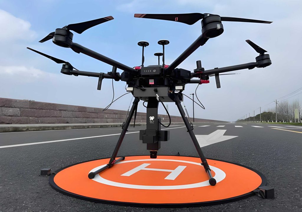
From my perspective, the most important technical gap is that many UAV drone communication studies assume a single antenna or assume that the UAV drone position is fixed and perfectly known. In practice, a UAV drone may move continuously, its exact position may be estimated with error, and the channel may contain both line-of-sight and non-line-of-sight components. These factors make conventional beamforming fragile. If the steering vector is mismatched, the beamformer may suppress the desired signal or fail to place a null toward an interferer. Similarly, if the UAV drone is deployed at an arbitrary or purely geometric center point, the transmit power required to satisfy all users may be much higher than necessary. I therefore develop a volume-integral Capon beamforming method and an improved firefly-based deployment method.
I begin with the communication channel. For a UAV drone operating at a moderate altitude, the air-to-ground channel is often modeled as a Rician channel because a dominant line-of-sight component usually exists, together with several weaker non-line-of-sight components. I write the channel between the UAV drone and ground user \(k\) as:
$$
\mathbf{h}_k=\sqrt{\beta_0 d_k^{-\alpha}}\mathbf{a}(\theta_k)
$$
where \(\beta_0\) is the channel gain at a reference distance, \(\alpha\) is the path-loss exponent, \(d_k\) is the distance between the UAV drone and user \(k\), and \(\mathbf{a}(\theta_k)\) is the array steering vector for the angle of departure or arrival. For a uniform linear array with \(M\) elements and element spacing \(d\), the steering vector is:
$$
\mathbf{a}(\theta)=\left[1,e^{-j\frac{2\pi d}{\lambda}\sin\theta},\ldots,e^{-j\frac{2\pi d}{\lambda}(M-1)\sin\theta}\right]^T
$$
Here, \(\lambda\) is the signal wavelength. I usually set \(d=\lambda/2\). This model allows me to express the UAV drone channel as a combination of large-scale fading and array response. In my simulations, I also consider the probability of line-of-sight and non-line-of-sight links. The line-of-sight probability can be written as:
$$
P_{\mathrm{LoS}}(\theta)=\frac{1}{1+a\exp(-b(\theta-a))}
$$
and the non-line-of-sight probability is \(1-P_{\mathrm{LoS}}(\theta)\). The elevation angle \(\theta\) between the UAV drone and the ground user strongly affects these probabilities. When the UAV drone is sufficiently high and has a clear view, the line-of-sight probability approaches one. The path loss for line-of-sight and non-line-of-sight links can be modeled separately, and the average path loss is:
$$
L(\theta)=P_{\mathrm{LoS}}(\theta)L_{\mathrm{LoS}}(\theta)+P_{\mathrm{NLoS}}(\theta)L_{\mathrm{NLoS}}(\theta)
$$
This modeling matters because the deployment of a UAV drone changes the elevation angle and distance to each ground user, which in turn changes the path loss and the required transmit power. I use this relationship later when I formulate the power-minimization problem.
For the interference suppression problem, I consider a UAV drone relay network in which the UAV drone receives a desired signal from a source base station and also receives multiple co-channel interference signals from other directions. The received signal at the UAV drone array can be written as:
$$
\mathbf{x}(k)=\mathbf{a}(\theta_0)s_0(k)+\sum_{l=1}^{P-1}\mathbf{a}(\theta_l)s_l(k)+\mathbf{n}(k)
$$
where \(\theta_0\) is the desired signal direction, \(\theta_l\) for \(l=1,\ldots,P-1\) are interference directions, \(s_0(k)\) is the desired signal envelope, \(s_l(k)\) are interference envelopes, and \(\mathbf{n}(k)\) is additive white Gaussian noise. The array output after applying the weight vector \(\mathbf{w}\) is:
$$
y(k)=\mathbf{w}^H\mathbf{x}(k)
$$
The covariance matrix of the received signal is:
$$
\mathbf{R}=E\{\mathbf{x}(k)\mathbf{x}^H(k)\}
=\sigma_0^2\mathbf{a}(\theta_0)\mathbf{a}^H(\theta_0)
+\sum_{l=1}^{P-1}\sigma_l^2\mathbf{a}(\theta_l)\mathbf{a}^H(\theta_l)
+\sigma_n^2\mathbf{I}
$$
I denote the interference-plus-noise covariance matrix by \(\mathbf{R}_{i+n}\). The Capon beamformer minimizes the output interference-plus-noise power subject to a distortionless response toward the desired signal:
$$
\min_{\mathbf{w}}\mathbf{w}^H\mathbf{R}_{i+n}\mathbf{w}
\quad
\mathrm{s.t.}
\quad
\mathbf{w}^H\mathbf{a}(\theta_0)=1
$$
The optimal weight vector is:
$$
\mathbf{w}_{\mathrm{opt}}=
\frac{\mathbf{R}_{i+n}^{-1}\mathbf{a}(\theta_0)}
{\mathbf{a}^H(\theta_0)\mathbf{R}_{i+n}^{-1}\mathbf{a}(\theta_0)}
$$
In practice, \(\mathbf{R}_{i+n}\) and \(\mathbf{a}(\theta_0)\) are not perfectly known. I estimate the covariance matrix from \(L\) snapshots:
$$
\hat{\mathbf{R}}=\frac{1}{L}\sum_{k=1}^{L}\mathbf{x}(k)\mathbf{x}^H(k)
$$
If I use \(\hat{\mathbf{R}}\) directly in the Capon formula, the desired signal may be present in the covariance matrix, especially at high input signal-to-noise ratio. This causes performance degradation. Also, if the steering vector is mismatched because of UAV drone movement or scattering, the beamformer may point away from the desired direction. To address these issues, I propose a volume-integral Capon beamforming algorithm.
The first step of my method is angle estimation. I use a root-MUSIC search instead of a conventional spectral MUSIC search. The covariance matrix can be decomposed into signal and noise subspaces:
$$
\mathbf{R}=\mathbf{U}_s\mathbf{\Sigma}_s\mathbf{U}_s^H+
\mathbf{U}_n\mathbf{\Sigma}_n\mathbf{U}_n^H
$$
The signal subspace is spanned by the steering vectors of the desired signal and the interferers, while the noise subspace is orthogonal to them. I define the polynomial:
$$
\mathbf{r}(z)=\mathbf{g}^T(z)\mathbf{c}_i,\quad
\mathbf{g}(z)=[1,z,\ldots,z^{M-1}]^T
$$
where \(\mathbf{c}_i\) belongs to the noise subspace. The roots of the polynomial that lie on the unit circle correspond to the signal directions. By solving for these roots, I obtain the desired angle \(\theta_0\) and the interference angles \(\theta_l\). This root-MUSIC step is important for a UAV drone because the UAV drone may move, and the angles of arrival change over time. A fast angle search allows the beamformer to update its nulls and main lobe in response to the current geometry.
After angle estimation, I reconstruct the interference-plus-noise covariance matrix. Rather than integrating the power spectrum only along a line or a surface, I perform a volume integral over a uncertainty set around the estimated interference steering vectors. I define a spherical uncertainty set:
$$
\mathcal{G}(\mathbf{a})=\{\mathbf{a}:\|\mathbf{a}-\bar{\mathbf{a}}\|_2\leq \epsilon\}
$$
and then combine the sets for all interference directions into a ring-like set:
$$
\mathcal{G}'(\mathbf{a})=\{\mathbf{a}:\|\mathbf{a}-\bar{\mathbf{a}}\|_2\leq \epsilon,\ \theta\in\hat{\Theta}_i\}
$$
The interference covariance matrix is reconstructed as a volume integral:
$$
\mathbf{R}_i=
\int_{\mathcal{G}'(\mathbf{a})}
\frac{\mathbf{a}\mathbf{a}^H}
{\mathbf{a}^H\mathbf{R}^{-1}\mathbf{a}}
\,dV
$$
In a practical implementation, I discretize the integral over angles and over the uncertainty surface:
$$
\hat{\mathbf{R}}_i
\approx
\sum_{m=1}^{M}
\sum_{n=1}^{N}
\frac{\mathbf{a}_{mn}\mathbf{a}_{mn}^H}
{\mathbf{a}_{mn}^H\mathbf{R}^{-1}\mathbf{a}_{mn}}
$$
I then approximate the noise covariance matrix by \(\lambda_M\mathbf{I}\), where \(\lambda_M\) is the smallest eigenvalue of \(\hat{\mathbf{R}}\). The interference-plus-noise covariance matrix is:
$$
\hat{\mathbf{R}}_{i+n}=\hat{\mathbf{R}}_i+\lambda_M\mathbf{I}
$$
The final step is to correct the desired steering vector. I solve:
$$
\min_{\mathbf{a}}
(\mathbf{a}-\bar{\mathbf{a}}_s)^H
\hat{\mathbf{R}}_{i+n}^{-1}
(\mathbf{a}-\bar{\mathbf{a}}_s)
\quad
\mathrm{s.t.}
\quad
\|\mathbf{a}-\bar{\mathbf{a}}_s\|_2^2\leq \varepsilon
$$
where \(\bar{\mathbf{a}}_s\) is the nominal steering vector obtained from the estimated desired angle. The corrected steering vector is then used to compute the beamforming weight:
$$
\mathbf{w}=
\frac{\hat{\mathbf{R}}_{i+n}^{-1}\hat{\mathbf{a}}}
{\hat{\mathbf{a}}^H\hat{\mathbf{R}}_{i+n}^{-1}\hat{\mathbf{a}}}
$$
I summarize the main beamforming categories that I considered in my research in the following table.
| Beamforming type | Key idea | Advantage | Limitation for UAV drone |
|---|---|---|---|
| Fixed beamforming | Weights are fixed; beams are switched among predefined directions | Low complexity and low cost | Poor adaptation to UAV drone mobility |
| Adaptive beamforming | Weights are updated according to a criterion | Strong interference suppression | Sensitive to steering vector mismatch |
| Analog beamforming | Phase shifters adjust the radio-frequency signal | Simple hardware at high frequency | Limited number of simultaneous beams |
| Digital beamforming | Baseband processing applies complex weights | Flexible, accurate, multiple beams | Higher hardware and power cost |
| Capon beamforming | Minimizes interference-plus-noise power with distortionless response | High resolution and good nulling | Requires accurate covariance and steering vector |
| Root-MUSIC based beamforming | Uses polynomial roots to estimate angles | Fast and accurate angle search | Still requires array calibration |
| Volume-integral Capon | Reconstructs covariance by volume integration | Robust to angle and scattering errors | Computational cost depends on discretization |
I evaluated the proposed beamformer through computer simulations. I used a uniform linear array with \(M=10\) elements and element spacing \(d=\lambda/2\). The desired signal was set at \(0^\circ\). Two interferers were placed at \(-30^\circ\) and \(40^\circ\). The interference-to-noise ratio was 30 dB. I compared my method with diagonal loading, a covariance-reconstruction method, and a steering-vector estimation method. I did not rely on perfect knowledge of the desired signal; instead, I used root-MUSIC to estimate the angles. The estimated angles were very close to the true angles, which confirms that the root-MUSIC step is suitable for a moving UAV drone.
The following table summarizes a representative angle-estimation result for the UAV drone relay scenario.
| Signal | True angle | Estimated angle | Absolute error |
|---|---|---|---|
| Desired signal | \(60^\circ\) | \(59.9589^\circ\) | \(0.0411^\circ\) |
| Interference 1 | \(10^\circ\) | \(9.8143^\circ\) | \(0.1857^\circ\) |
| Interference 2 | \(20^\circ\) | \(20.1415^\circ\) | \(0.1415^\circ\) |
I also studied the normalized beam pattern. My volume-integral Capon method placed the main lobe toward the desired direction and formed deep nulls toward the interferers. The diagonal loading method was less effective at high signal-to-noise ratio because the desired signal remained in the covariance matrix. The covariance-reconstruction method had a lower side-lobe level than diagonal loading, but its main lobe was sometimes shifted when the steering vector was mismatched. My method maintained a stable main lobe and deep nulls because the volume integral collected potential errors around the interference directions and reconstructed a more accurate interference-plus-noise covariance matrix.
Next, I examined the output signal-to-interference-plus-noise ratio, which I define as:
$$
\mathrm{SINR}=
\frac{\sigma_s^2|\mathbf{w}^H\mathbf{a}(\theta_0)|^2}
{\mathbf{w}^H\mathbf{R}_{i+n}\mathbf{w}}
$$
I varied the input signal-to-noise ratio from \(-20\) dB to \(20\) dB and fixed the number of snapshots at 100. I observed that my method achieved a higher output SINR than diagonal loading over the entire range. At low input SNR, my method performed close to the best available method because the volume integral reduced the effect of noise and steering-vector uncertainty. At high input SNR, my method remained stable, while diagonal loading degraded because the desired signal was included in the covariance estimate. The covariance-reconstruction method also degraded at high SNR, but less severely. My method was the most robust across the tested range.
I then fixed the input SNR at 10 dB and varied the number of snapshots. My method converged quickly and approached the optimal SINR with fewer snapshots than the other methods. The diagonal loading method showed poor convergence and even degraded as the number of snapshots increased, because the desired signal component became more dominant in the sample covariance matrix. My method used root-MUSIC to identify the interference angles and then reconstructed the covariance over a restricted uncertainty set, so it did not need a very large number of snapshots to obtain a good estimate. This is important for a UAV drone, because the UAV drone may not have enough time or computational resources to collect a large number of snapshots before updating its beamformer.
I also tested the effect of the number of interferers. As the number of interferers increased, my method maintained a higher output SINR than the comparison methods. Diagonal loading and the covariance-reconstruction method showed noticeable performance loss when more interferers were present. The volume-integral method was more tolerant because it reconstructed the interference covariance over a union of angular regions rather than relying on a small number of exact interference directions. The following table summarizes the qualitative performance comparison.
| Method | Main-lobe accuracy | Null depth | Robustness to SNR | Robustness to snapshots | Robustness to many interferers |
|---|---|---|---|---|---|
| Diagonal loading | Medium | Weak | Low | Low | Low |
| Covariance reconstruction | Medium | Medium | Medium | Medium | Medium |
| Steering-vector estimation | Medium | Strong | Medium | Medium | Medium |
| Volume-integral Capon | High | Strong | High | High | High |
After addressing interference suppression, I turned to the second major problem: optimized deployment of a multi-antenna UAV drone. I consider a scenario in which a UAV drone acts as a temporary base station for \(K\) ground users. Each ground user is single-antenna, and the UAV drone is equipped with a uniform linear array of \(M\) antennas. The UAV drone transmits independent data streams to the users through digital beamforming. I use zero-forcing beamforming at the transmitter because it is simple, has low complexity, and can cancel inter-user interference when \(M\geq K\). The channel matrix between the UAV drone and the users is:
$$
\mathbf{H}=[\mathbf{h}_1,\mathbf{h}_2,\ldots,\mathbf{h}_K]\in\mathbb{C}^{M\times K}
$$
The zero-forcing beamforming matrix is:
$$
\mathbf{W}=\mathbf{H}^H(\mathbf{H}\mathbf{H}^H)^{-1}
$$
I normalize each column of \(\mathbf{W}\) to obtain the beamforming vector for each user. The received signal at user \(k\) is:
$$
y_k=\mathbf{h}_k^H\mathbf{w}_k\sqrt{p_k}s_k
+\sum_{i\in I\setminus\{k\}}\mathbf{h}_k^H\mathbf{w}_i\sqrt{p_i}s_i
+n_k
$$
The achievable rate of user \(k\) is:
$$
C_k=
B\log_2\left(
1+
\frac{p_k|\mathbf{h}_k^H\mathbf{w}_k|^2}
{\sum_{i\in I\setminus\{k\}}p_i|\mathbf{h}_k^H\mathbf{w}_i|^2+\sigma_n^2}
\right)
$$
With zero-forcing beamforming, the inter-user interference is suppressed, and the rate expression simplifies to:
$$
C_k=
B\log_2\left(
1+
\frac{p_k M d_k^{-\alpha}\beta_0}{\sigma_n^2}
\right)
$$
Therefore, the transmit power required by user \(k\) for a target rate \(c_k\) is:
$$
p_k=
\frac{\sigma_n^2 d_k^{\alpha}}{M\beta_0}
\left(2^{c_k/B}-1\right)
$$
The total transmit power of the UAV drone is:
$$
P_{\mathrm{total}}=
\sum_{k=1}^{K}p_k
=
\sum_{k=1}^{K}
\frac{\sigma_n^2 d_k^{\alpha}}{M\beta_0}
\left(2^{c_k/B}-1\right)
$$
I formulate the deployment optimization problem as:
$$
\min_{x_u,y_u}
P_{\mathrm{total}}
$$
$$
\mathrm{s.t.}\quad
C_k\geq c_k,\quad \forall k
$$
$$
x_{\min}\leq x_u\leq x_{\max},
\quad
y_{\min}\leq y_u\leq y_{\max}
$$
where \((x_u,y_u)\) is the horizontal position of the UAV drone, and \(c_k\) is the minimum required rate of user \(k\). Because the total power decreases as the UAV drone moves closer to the users, the optimal deployment is not necessarily the geometric center of the user distribution. I therefore need a fast search algorithm that can find a UAV drone position that satisfies all rate constraints while minimizing the total transmit power.
The standard firefly algorithm is a metaheuristic algorithm inspired by the flashing behavior of fireflies. Each firefly represents a candidate UAV drone position. The brightness of a firefly is related to the objective function value. A firefly is attracted to brighter fireflies, and its movement is affected by distance and attractiveness. The distance between two fireflies is:
$$
r_{ij}=\|\mathbf{x}_i-\mathbf{x}_j\|
$$
The brightness of firefly \(j\) as seen by firefly \(i\) is:
$$
I_{ij}=I_j e^{-\gamma r_{ij}^2}
$$
The attractiveness is:
$$
\beta_{ij}=\beta_0 e^{-\gamma r_{ij}^2}
$$
The basic position update is:
$$
\mathbf{x}_i(t+1)=
\mathbf{x}_i(t)+
\beta_{ij}(\mathbf{x}_j(t)-\mathbf{x}_i(t))
+\alpha(\mathrm{rand}-0.5)
$$
Although the firefly algorithm is simple and has few parameters, it can converge too quickly to a local optimum and may have slow convergence in the later stage. I therefore propose a firefly algorithm based on inertia weight and dynamic step, which I call FABD. I add an inertia term that represents the attraction of the best firefly in the current population:
$$
\mathbf{x}_i(t+1)=
\mathbf{x}_i(t)+
\beta_{ij}(\mathbf{x}_j(t)-\mathbf{x}_i(t))
+\alpha(t)(\mathrm{rand}-0.5)
+\omega_i(t)(\mathbf{x}_{\mathrm{best}}(t)-\mathbf{x}_i(t))
$$
The inertia weight \(\omega_i(t)\) is designed to be adaptive. It depends on the best objective value, the mean objective value, and the previous two objective values of firefly \(i\):
$$
\omega_i(t)=
\exp\left[
-\left(
\frac{f_{\mathrm{best}}(t)-f_i(t-1)}
{M_f(t)-f_i(t-2)}
\right)^2
\right]
$$
The dynamic step is:
$$
\alpha(t)=\alpha_0\delta^t,\quad 0<\delta<1
$$
This dynamic step is large in the early iterations, which helps the algorithm explore the deployment area, and it becomes smaller in later iterations, which helps the algorithm converge precisely. The inertia term helps the population follow the best candidate position but still allows local search through the random term.
I tested the deployment algorithm in a \(500\,\mathrm{m}\times500\,\mathrm{m}\) area. The UAV drone altitude was fixed at \(100\,\mathrm{m}\). I used \(K=4\) ground users and \(M=10\) antennas. The bandwidth was \(1\,\mathrm{MHz}\). The reference channel gain was \(1.42\times10^{-4}\), and the path-loss exponent was \(3.8\). The ground users were randomly placed, and their minimum rate requirements were different. I compared FABD with the standard firefly algorithm, ant colony optimization, and particle swarm optimization. I also compared the optimized deployment with the area center and two random deployment positions. The following table lists the main simulation parameters.
| Parameter | Value |
|---|---|
| Area size | \(500\,\mathrm{m}\times500\,\mathrm{m}\) |
| UAV drone altitude | \(100\,\mathrm{m}\) |
| Number of ground users | \(K=4\) |
| Number of UAV drone antennas | \(M=10\) |
| Bandwidth | \(B=1\,\mathrm{MHz}\) |
| Reference channel gain | \(\beta_0=1.42\times10^{-4}\) |
| Path-loss exponent | \(\alpha=3.8\) |
| User rate requirements | 1.4384, 2.2342, 1.3295, 3.8346 Mbit/s |
I first studied the convergence behavior. With a population size of 10, FABD converged in about 17 iterations, while the standard firefly algorithm converged in about 20 iterations. Ant colony optimization converged in about 24 iterations, and particle swarm optimization converged in about 28 iterations. When I increased the population size to 20, all algorithms converged faster, but FABD still required the fewest iterations. This shows that the inertia weight and dynamic step improve both the exploration speed and the convergence stability. The following table summarizes the average number of iterations under different population sizes.
| Population size | FABD | Standard firefly | Ant colony optimization | Particle swarm optimization |
|---|---|---|---|---|
| 10 | 17 | 20 | 24 | 28 |
| 20 | 10 | 13 | 14 | 19 |
I also compared the deployment positions obtained by the different methods. The standard firefly algorithm produced a UAV drone position near \((357.5254,215.3677,100)\). FABD produced a position near \((350.1715,208.8123,100)\). Ant colony optimization produced a position near \((332.0064,205.1268,100)\), and particle swarm optimization produced a position near \((317.5714,195.2793,100)\). Although these positions are not identical, they all reflect the trade-off between distance to the users and the rate requirements. FABD moved more directly toward the best region in the early iterations because the inertia term pulled the population toward the best candidate. The standard firefly algorithm relied more heavily on the random term, so it required more iterations to reach a similar accuracy.
I then compared the total transmit power for different deployment positions. I included the area center and two random positions as baselines. The optimized positions obtained by FABD and the standard firefly algorithm required much lower power than the center and random positions. FABD consistently achieved the lowest total power. The following table gives a representative comparison for a fixed set of parameters.
| Deployment position | Horizontal coordinates | Total transmit power | Relative performance |
|---|---|---|---|
| Area center | \((250,250)\) | High | Baseline |
| Random position 1 | \((180,320)\) | High | Poor |
| Random position 2 | \((430,80)\) | Very high | Very poor |
| Standard firefly | \((357.53,215.37)\) | Low | Good |
| FABD | \((350.17,208.81)\) | Lowest | Best |
I also examined how the total transmit power changes with the number of UAV drone antennas. As \(M\) increases, the total power decreases because the array gain increases. However, the improvement becomes gradual after \(M=30\). This means that adding more antennas is beneficial, but the UAV drone must also consider payload, radio-frequency chain power, and computational complexity. The optimized deployment remains better than the center or random deployment across all antenna numbers. The following table summarizes the trend.
| Number of antennas \(M\) | Power trend | Deployment advantage of FABD |
|---|---|---|
| 5 | High | Noticeable |
| 10 | Medium | Noticeable |
| 20 | Lower | Moderate |
| 30 | Low | Slight but consistent |
| 40 | Very low | Slight but consistent |
Next, I studied the effect of the path-loss exponent. As the path-loss exponent increases, the UAV drone must transmit more power to compensate for the additional attenuation. The total power increases roughly exponentially with the path-loss exponent. The FABD deployment remains superior to the standard firefly deployment, and both are much better than the center and random deployments. When the path-loss exponent is below 3.8, the difference between FABD and the standard firefly algorithm is small. When the path-loss exponent is above 3.8, FABD becomes clearly better. This is because the inertia weight helps the algorithm avoid local optima when the objective function becomes steeper.
I also analyzed the relationship between total transmit power and the minimum user rate. As the required rate increases, the UAV drone must allocate more power to each user. The total power increases accordingly. FABD again requires less power than the comparison methods. This confirms that deployment optimization is not only a coverage problem but also an energy problem. A well-placed UAV drone can reduce the power needed to satisfy the same rate requirements, which extends the operational time of the UAV drone.
From my perspective, the combination of volume-integral Capon beamforming and FABD deployment provides a coherent solution for UAV drone-assisted communication. Beamforming addresses the spatial dimension: it increases the desired signal gain and suppresses interference. Deployment addresses the geometric dimension: it places the UAV drone where the channel conditions are favorable for all users. Together, they reduce the power consumption of the UAV drone while maintaining communication quality. The following table summarizes the overall design.
| Problem | Proposed method | Main benefit | Key metric |
|---|---|---|---|
| Interference and steering-vector mismatch | Volume-integral Capon beamforming with root-MUSIC | Robust nulling and main-lobe accuracy | Output SINR |
| Slow convergence and local optima in deployment | FABD with inertia weight and dynamic step | Fast convergence and lower transmit power | Total transmit power |
| Multi-user interference | Zero-forcing digital beamforming | Inter-user interference cancellation | Achievable rate |
| UAV drone endurance | Power-minimized deployment | Longer communication time | Power consumption |
I also want to emphasize the practical implications for a UAV drone. A UAV drone cannot rely on a fixed power supply, so every Watt matters. If the beamformer is not robust, the UAV drone may waste power by transmitting in the wrong direction or by amplifying interference. If the deployment is poor, the UAV drone may need to increase power to compensate for distance and path loss. My research shows that robust beamforming and optimized deployment are not separate improvements; they are complementary. A robust beamformer makes the effective channel more predictable, and an optimized deployment makes the beamformer’s job easier by improving the geometry.
In my beamforming simulations, I observed that the volume-integral method achieved deep nulls toward interferers and maintained a stable main lobe even when the desired steering vector was not perfectly known. The root-MUSIC step was accurate enough to identify the desired and interference angles under the tested conditions. The output SINR improved as the number of snapshots increased, but the method converged quickly and did not require an excessively large number of snapshots. This is important for a UAV drone because the radio environment may change rapidly as the UAV drone moves. The method also handled multiple interferers better than the comparison methods, which suggests that it can be used in dense interference environments.
In my deployment simulations, I observed that FABD converged faster than the standard firefly algorithm and the other metaheuristics. The inertia weight allowed the population to follow the best candidate position without losing diversity too early. The dynamic step allowed the algorithm to explore the area in the early iterations and refine the position in the later iterations. The optimized UAV drone position reduced the total transmit power compared with the area center and random positions. The advantage remained consistent when I changed the number of antennas, the path-loss exponent, and the minimum rate requirements. This indicates that the proposed deployment method is robust to different operating conditions.
I now describe the main steps of my deployment method in more detail. First, I initialize the coverage area, the number of ground users, their positions, their minimum rate requirements, the firefly population size, the number of iterations, the maximum attractiveness, the light absorption coefficient, the initial step size, and the scaling factor. Second, I randomly place the fireflies within the coverage area. Each firefly represents a candidate horizontal position for the UAV drone. Third, I compute the brightness of each firefly from the total transmit power expression. A lower total power corresponds to a higher brightness. Fourth, I update the position of each firefly using the FABD position update equation. Fifth, I check whether the termination condition is satisfied. If not, I repeat the position update. Finally, I output the best UAV drone position and the corresponding total transmit power.
The following algorithm table summarizes the FABD procedure.
| Step | Operation |
|---|---|
| 1 | Initialize area, users, rate requirements, population, iterations, and algorithm parameters |
| 2 | Randomly place fireflies in the UAV drone coverage area |
| 3 | Compute the brightness of each firefly using the total power objective |
| 4 | Determine the movement direction and distance based on attractiveness |
| 5 | Update the position and brightness of each firefly using inertia weight and dynamic step |
| 6 | Check the termination condition |
| 7 | Output the best UAV drone position and minimum total transmit power |
I also consider the computational complexity. The volume-integral Capon method is more complex than diagonal loading because it reconstructs the covariance matrix over a discretized uncertainty set. However, the root-MUSIC step reduces the angular search range, and the volume integral can be limited to the estimated interference regions. The FABD algorithm is also more complex than the standard firefly algorithm because it adds an inertia term, but the additional computation is small compared with the benefit of faster convergence and lower transmit power. For a UAV drone with limited onboard computing resources, this trade-off is acceptable because the deployment can be computed before or during the mission, and the beamforming weights can be updated at a lower rate than the data transmission.
I summarize the key formulas of my framework in one place for clarity. The array steering vector is:
$$
\mathbf{a}(\theta)=
\left[
1,e^{-j\frac{2\pi d}{\lambda}\sin\theta},
\ldots,
e^{-j\frac{2\pi d}{\lambda}(M-1)\sin\theta}
\right]^T
$$
The received signal model is:
$$
\mathbf{x}(k)=\mathbf{a}(\theta_0)s_0(k)+\sum_{l=1}^{P-1}\mathbf{a}(\theta_l)s_l(k)+\mathbf{n}(k)
$$
The covariance matrix is:
$$
\mathbf{R}=
\sigma_0^2\mathbf{a}(\theta_0)\mathbf{a}^H(\theta_0)
+\sum_{l=1}^{P-1}\sigma_l^2\mathbf{a}(\theta_l)\mathbf{a}^H(\theta_l)
+\sigma_n^2\mathbf{I}
$$
The Capon weight is:
$$
\mathbf{w}_{\mathrm{opt}}=
\frac{\mathbf{R}_{i+n}^{-1}\mathbf{a}(\theta_0)}
{\mathbf{a}^H(\theta_0)\mathbf{R}_{i+n}^{-1}\mathbf{a}(\theta_0)}
$$
The reconstructed interference covariance is:
$$
\hat{\mathbf{R}}_i
\approx
\sum_{m=1}^{M}
\sum_{n=1}^{N}
\frac{\mathbf{a}_{mn}\mathbf{a}_{mn}^H}
{\mathbf{a}_{mn}^H\mathbf{R}^{-1}\mathbf{a}_{mn}}
$$
The SINR is:
$$
\mathrm{SINR}=
\frac{\sigma_s^2|\mathbf{w}^H\mathbf{a}(\theta_0)|^2}
{\mathbf{w}^H\mathbf{R}_{i+n}\mathbf{w}}
$$
The zero-forcing beamforming matrix is:
$$
\mathbf{W}=\mathbf{H}^H(\mathbf{H}\mathbf{H}^H)^{-1}
$$
The achievable rate is:
$$
C_k=
B\log_2\left(
1+
\frac{p_k|\mathbf{h}_k^H\mathbf{w}_k|^2}
{\sum_{i\in I\setminus\{k\}}p_i|\mathbf{h}_k^H\mathbf{w}_i|^2+\sigma_n^2}
\right)
$$
The simplified rate with zero-forcing is:
$$
C_k=
B\log_2\left(
1+
\frac{p_k M d_k^{-\alpha}\beta_0}{\sigma_n^2}
\right)
$$
The required power per user is:
$$
p_k=
\frac{\sigma_n^2 d_k^{\alpha}}{M\beta_0}
\left(2^{c_k/B}-1\right)
$$
The total power is:
$$
P_{\mathrm{total}}=
\sum_{k=1}^{K}
\frac{\sigma_n^2 d_k^{\alpha}}{M\beta_0}
\left(2^{c_k/B}-1\right)
$$
The deployment optimization is:
$$
\min_{x_u,y_u}
P_{\mathrm{total}}
$$
$$
\mathrm{s.t.}\quad
C_k\geq c_k,\quad
x_{\min}\leq x_u\leq x_{\max},\quad
y_{\min}\leq y_u\leq y_{\max}
$$
The FABD position update is:
$$
\mathbf{x}_i(t+1)=
\mathbf{x}_i(t)+
\beta_{ij}(\mathbf{x}_j(t)-\mathbf{x}_i(t))
+\alpha(t)(\mathrm{rand}-0.5)
+\omega_i(t)(\mathbf{x}_{\mathrm{best}}(t)-\mathbf{x}_i(t))
$$
The inertia weight is:
$$
\omega_i(t)=
\exp\left[
-\left(
\frac{f_{\mathrm{best}}(t)-f_i(t-1)}
{M_f(t)-f_i(t-2)}
\right)^2
\right]
$$
The dynamic step is:
$$
\alpha(t)=\alpha_0\delta^t,\quad 0<\delta<1
$$
In my view, the most interesting insight is that the two problems are linked by the UAV drone position. The position determines the distances \(d_k\), the angles \(\theta_k\), the path loss, and the steering vectors. Therefore, the beamforming performance and the power consumption both depend on the deployment. Conversely, the beamforming design determines how much spatial gain the UAV drone can obtain, which affects how much transmit power is needed to satisfy the rate constraints. A joint design is more effective than treating beamforming and deployment as independent problems. My framework does not fully solve the joint optimization in one step, but it provides a practical decomposition: use robust beamforming to handle interference and angle uncertainty, and use FABD to minimize transmit power while satisfying rate constraints.
I also note some limitations of my study. I assumed that the ground users are single-antenna. If the ground users are equipped with multiple antennas, they could obtain receive diversity or spatial multiplexing gains, which would change the rate and power expressions. I also assumed that the UAV drone position is known for the deployment optimization. In practice, the UAV drone position may be estimated with error, which could affect the channel model and the beamforming weights. In addition, I did not explicitly model the backhaul link between the UAV drone and the core network. The backhaul power could be significant in some scenarios, especially if the UAV drone must relay data over a long distance. These limitations suggest several directions for future work.
For future work, I would like to extend the channel model to include Doppler effects caused by UAV drone mobility. A moving UAV drone can induce a Doppler shift, which affects the coherence time and the channel estimation. I would also like to study ground users with multiple antennas and evaluate how receive beamforming interacts with the UAV drone transmit beamforming. Another direction is to include the backhaul link in the power minimization problem, so that the total power includes both access and backhaul transmission. Finally, I would like to test the proposed methods in more realistic environments with obstacles, shadowing, and dynamic interference. These extensions would make the framework more complete and closer to practical deployment.
Overall, my research shows that a UAV drone can provide flexible and reliable wireless service when terrestrial infrastructure is unavailable. By combining multi-antenna beamforming with optimized deployment, the UAV drone can suppress interference, improve the desired signal gain, and reduce transmit power. The volume-integral Capon beamforming method is robust to steering-vector mismatch and multiple interferers, and the FABD algorithm converges quickly to a low-power deployment. I believe these contributions are useful for emergency communication, temporary coverage, and future integrated air-ground networks.