
In recent years, the proposal of the low-altitude economy has renewed focus and spurred the application of unmanned aerial vehicles (UAVs). Among these, the quadrotor drone stands out due to its advantages of low cost, vertical take-off and landing, and aerial hovering. However, the quadrotor drone is a highly unstable system. A sensitive, robust trajectory tracking and stable flight control system is the key prerequisite for executing flight missions, placing higher demands on tracking accuracy. Model parameter uncertainties, unmodeled system dynamics, and other internal adverse factors often lead to unsatisfactory control performance for methods reliant on precise models. Simultaneously, external disturbances such as strong wind gusts and sensor noise further increase the difficulty of controller design. Therefore, designing a robust controller for a quadrotor drone remains a significant challenge in this research field.
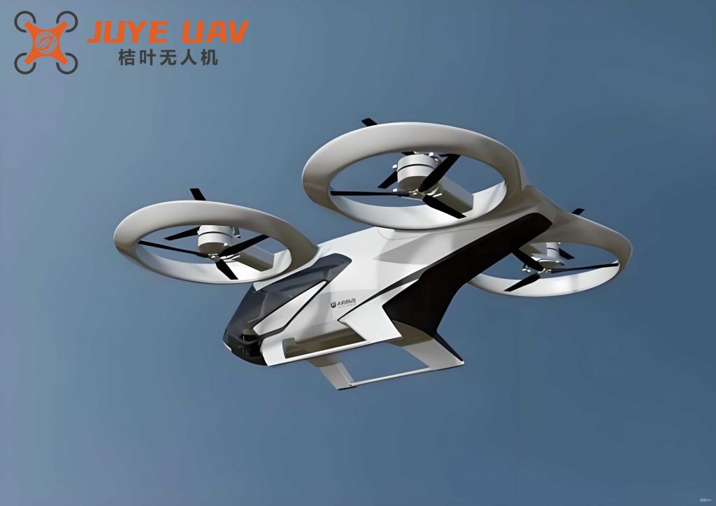
Disturbance rejection control, owing to its ability to suppress disturbances, has been widely applied to quadrotor drones. Generally, disturbance rejection control can be categorized into two classes: one involves designing robust controllers to achieve disturbance rejection; the other involves designing disturbance observers to estimate and compensate for disturbances. The first class includes methods based on the “industrial paradigm” of classical control theory—error elimination based on error—such as PID and Linear Quadratic Regulator (LQR). These linear control methods have simple structures and are easy to implement, but they often suffer from weak disturbance rejection and limited control accuracy. The second class, based on the “model paradigm” of modern control theory, describes internal mechanisms. For instance, Model Predictive Control (MPC) can handle dynamics and input saturation constraints for UAV trajectory tracking, but it is computationally intensive. These methods, relying on model linearization and nominal mathematical models, can achieve disturbance rejection for low-energy disturbances through the inherent robustness of their algorithms.
However, as quadrotor drones face increasing complexity and diversity in mission execution while being subjected to multi-source disturbances, the aforementioned methods often struggle to meet the requirements for active disturbance suppression. A prevalent approach, as seen in the literature, is to design disturbance observers to estimate disturbances and then feed the estimated information forward into the controller for active and rapid disturbance rejection. For example, high-order sliding mode observers or nonlinear disturbance observers have been used to estimate lumped disturbances in systems. Combining nonlinear disturbance observers with sliding mode control can further enhance system robustness. These methods design observers based on assumptions about the disturbance’s characteristics, yet their robustness in guaranteeing rapid, active suppression may be insufficient when disturbances are unknown or have high energy.
Active Disturbance Rejection Control (ADRC) represents an anti-disturbance approach based on the Extended State Observer (ESO). Its core idea is to treat both internal and external disturbances as a lumped disturbance, estimate it in real-time via the ESO, and compensate for it, forming an “anti-disturbance paradigm.” However, many existing applications of ADRC on quadrotor drones primarily use the ESO to estimate the lumped disturbance combined with a simple PD controller, which inherently faces a trade-off between response speed and overshoot. Furthermore, these applications often do not fully exploit the ESO’s capability to estimate system state information, which could enable sensorless velocity control.
To address these limitations and enhance the trajectory tracking accuracy and rapidity of a quadrotor drone under multi-source disturbances, this work proposes a composite control scheme. This scheme integrates a Global Non-singular Fast Terminal Sliding Mode Control (GNFTSMC) with an ESO, forming a Composite Global Non-singular Fast Terminal Sliding Mode Control (CGNFTSMC). The design process carefully considers the characteristics of the quadrotor drone’s position and attitude loops.
The main contributions of this article are summarized as follows:
1. The underactuated quadrotor drone system is decomposed into four independent channels: the altitude channel, the yaw channel, and two cascade channels (horizontal X-pitch and horizontal Y-roll). A virtual control law is introduced to facilitate this decoupling.
2. An ESO is designed for each channel to simultaneously estimate the lumped disturbance (encompassing couplings and external disturbances) and the system’s state information (e.g., velocity). This enables active disturbance compensation and paves the way for potential sensorless control.
3. Based on the estimated information from the ESO and the smooth reference signals provided by Tracking Differentiators (TDs), a composite global non-singular fast terminal sliding mode controller is designed for each channel. The saturation function replaces the sign function to ensure control signal continuity.
4. The stability of the closed-loop system, including the convergence of the ESO and the finite-time convergence of the tracking error, is rigorously proven using Lyapunov theory.
5. Extensive comparative simulations demonstrate the superior performance of the proposed CGNFTSMC method over traditional PID, ADRC (with PD), and standard NFTSMC without an observer, in terms of tracking accuracy and disturbance rejection.
System Modeling and Problem Formulation for the Quadrotor Drone
Mathematical Model of the Quadrotor Drone
To improve the maneuverability of the quadrotor drone, an “X”-configuration is chosen as the research object. Two coordinate frames are defined: the body-fixed frame \(O_bX_bY_bZ_b\) and the inertial frame \(O_eX_eY_eZ_e\). The following standard assumptions are made: 1) The quadrotor drone is a rigid body, uniform and symmetric; 2) The system mass and moments of inertia are constant; 3) The geometric center coincides with the center of mass.
Let the position and velocity vectors in the inertial frame be \(\mathbf{P} = [x, y, z]^T\) and \(\dot{\mathbf{P}} = [\dot{x}, \dot{y}, \dot{z}]^T\), respectively. The attitude angles (roll \(\phi\), pitch \(\theta\), yaw \(\psi\)) are represented by \(\mathbf{\Theta} = [\phi, \theta, \psi]^T\), and the angular velocities in the body frame by \(\dot{\mathbf{\Theta}} = [\dot{\phi}, \dot{\theta}, \dot{\psi}]^T\). Using the Newton-Euler formulation, the dynamic model of the quadrotor drone is established as follows:
$$
\begin{align}
\ddot{x} &= (\cos\phi \sin\theta \cos\psi + \sin\phi \sin\psi)\frac{f}{m} – \frac{k_1}{m}\dot{x} + d_1 \\
\ddot{y} &= (\cos\phi \sin\theta \sin\psi – \sin\phi \cos\psi)\frac{f}{m} – \frac{k_2}{m}\dot{y} + d_2 \\
\ddot{z} &= g – (\cos\phi \cos\theta)\frac{f}{m} – \frac{k_3}{m}\dot{z} + d_3 \\
\ddot{\phi} &= \dot{\theta}\dot{\psi}\left(\frac{I_y – I_z}{I_x}\right) + \frac{l}{I_x}\tau_x – \frac{k_4}{I_x}\dot{\phi} + d_4 \\
\ddot{\theta} &= \dot{\phi}\dot{\psi}\left(\frac{I_z – I_x}{I_y}\right) + \frac{l}{I_y}\tau_y – \frac{k_5}{I_y}\dot{\theta} + d_5 \\
\ddot{\psi} &= \dot{\phi}\dot{\theta}\left(\frac{I_x – I_y}{I_z}\right) + \frac{1}{I_z}\tau_z – \frac{k_6}{I_z}\dot{\psi} + d_6
\end{align}
$$
where \(f\) is the total thrust generated by the four rotors; \(m\) is the mass; \(g\) is gravitational acceleration; \(I_x, I_y, I_z\) are the moments of inertia; \(\boldsymbol{\tau} = [\tau_x, \tau_y, \tau_z]^T\) are the control moments; \(k_1, k_2, k_3\) are translational drag coefficients; \(k_4, k_5, k_6\) are rotational drag coefficients; \(d_i (i=1,…,6)\) represent external disturbances; and \(l\) is the arm length from the center to each rotor.
The relationship between the total thrust/moments and the squares of the rotor speeds \(\varpi_i^2\) (for rotors i=1,2,3,4) for the “X”-configuration is:
$$
\begin{align}
f &= C_T (\varpi_1^2 + \varpi_2^2 + \varpi_3^2 + \varpi_4^2) \\
\tau_x &= \frac{\sqrt{2}}{2} l C_T (-\varpi_1^2 – \varpi_2^2 + \varpi_3^2 + \varpi_4^2) \\
\tau_y &= \frac{\sqrt{2}}{2} l C_T (-\varpi_1^2 + \varpi_2^2 + \varpi_3^2 – \varpi_4^2) \\
\tau_z &= C_M (\varpi_1^2 + \varpi_2^2 – \varpi_3^2 – \varpi_4^2)
\end{align}
$$
where \(C_T\) is the thrust coefficient and \(C_M\) is the torque coefficient.
Problem Formulation and Channel Decoupling
Considering the underactuated nature of the quadrotor drone, the system is divided into four independent channels: the altitude (Z) channel, the yaw (\(\psi\)) channel, the cascade X-\(\theta\) channel, and the cascade Y-\(\phi\) channel. The control allocation is shown in the conceptual diagram below.
Virtual control inputs are introduced for the position loop:
$$
\begin{align}
u_x &= (\cos\phi \sin\theta \cos\psi + \sin\phi \sin\psi)f \\
u_y &= (\cos\phi \sin\theta \sin\psi – \sin\phi \cos\psi)f \\
u_z &= (\cos\phi \cos\theta)f
\end{align}
$$
Substituting these into the translational dynamics yields a simpler form:
$$
\begin{align}
\ddot{x} &= u_x / m + D_x, \quad \ddot{y} = u_y / m + D_y, \quad \ddot{z} = u_z / m + D_z \\
\ddot{\phi} &= \tau_x / I_x + D_{\phi}, \quad \ddot{\theta} = \tau_y / I_y + D_{\theta}, \quad \ddot{\psi} = \tau_z / I_z + D_{\psi}
\end{align}
$$
Here, \(D_x, D_y, D_z, D_{\phi}, D_{\theta}, D_{\psi}\) represent the lumped disturbances for each channel, which include couplings (e.g., \(\dot{\theta}\dot{\psi}(I_y-I_z)/I_x\)), linear/nonlinear damping terms (\(-k_i\dot{(\cdot)}\)), and external disturbances (\(d_i\)). For example, \(D_x = -(k_1/m)\dot{x} + d_1\).
The required total thrust \(f_d\) and desired attitude angles \(\phi_d, \theta_d\) can be solved from the virtual controls and the desired yaw angle \(\psi_d\):
$$
\begin{align}
f_d &= \frac{u_z}{\cos\phi_d \cos\theta_d} \\
\theta_d &= \arctan\left(\frac{u_x \cos\psi_d + u_y \sin\psi_d}{u_z}\right) \\
\phi_d &= \arctan\left(\frac{u_x \sin\psi_d – u_y \cos\psi_d}{u_z}\right)
\end{align}
$$
Defining the trajectory tracking errors as \(e_x = x_d – x\), \(e_y = y_d – y\), \(e_z = z_d – z\), \(e_{\phi} = \phi_d – \phi\), \(e_{\theta} = \theta_d – \theta\), \(e_{\psi} = \psi_d – \psi\), and their derivatives, the control objective is transformed into stabilizing these tracking errors to zero.
Design of the Composite Controller for the Quadrotor Drone
The proposed CGNFTSMC scheme integrates several components: a Tracking Differentiator (TD) to provide smooth reference signals and their derivatives, an Extended State Observer (ESO) to estimate state information and lumped disturbances, and a Non-singular Fast Terminal Sliding Mode Controller (NFTSMC) that uses the estimates for robust control. Due to structural symmetry, the design for the yaw channel is presented as an illustrative example. The control structure is shown below conceptually.
Controller Design for the Altitude Channel
The altitude channel is an independent channel responsible for generating the thrust control \(f_d\).
1. Cascade Tracking Differentiator (TD):
A second-order TD is used to track the desired altitude \(z_d\) and obtain its smooth derivatives.
$$
\begin{align}
\dot{v}_{z1} &= v_{z2} \\
\dot{v}_{z2} &= \text{fhan}(v_{z1} – z_d, v_{z2}, r_{z1}, h_0) \\
\dot{v}_{z3} &= v_{z4} \\
\dot{v}_{z4} &= \text{fhan}(v_{z3} – v_{z2}, v_{z4}, r_{z2}, h_0)
\end{align}
$$
Here, \(v_{z1}\) tracks \(z_d\), \(v_{z2}\) is the estimated first derivative, and \(v_{z4}\) is the estimated second derivative. \(r_{z1}, r_{z2}\) are speed factors, \(h_0\) is the filter factor, and \(\text{fhan}(\cdot)\) is the optimal control synthesis function.
2. Extended State Observer (ESO) for Altitude:
A third-order ESO is designed for the altitude subsystem \(\ddot{z} = b_{0z} u_z + D_z\), where \(b_{0z} = 1/m\). Let \(z_1 = z\), \(z_2 = \dot{z}\), and \(z_3 = D_z\) be the extended state representing the lumped disturbance.
$$
\begin{align}
\dot{\hat{z}}_1 &= \hat{z}_2 + \beta_{11z}(z – \hat{z}_1) \\
\dot{\hat{z}}_2 &= \hat{z}_3 + b_{0z} u_z + \beta_{12z}(z – \hat{z}_1) \\
\dot{\hat{z}}_3 &= \beta_{13z}(z – \hat{z}_1)
\end{align}
$$
where \(\beta_{11z}, \beta_{12z}, \beta_{13z}\) are observer gains tuned via the bandwidth parameter \(\omega_{oz}\): \(\beta_{11z} = 3\omega_{oz}, \beta_{12z} = 3\omega_{oz}^2, \beta_{13z} = \omega_{oz}^3\). The estimates are \(\hat{z} \approx z\), \(\hat{\dot{z}} \approx \dot{z}\), and \(\hat{D}_z \approx D_z\).
3. Non-singular Fast Terminal Sliding Mode Controller (NFTSMC):
Define a global non-singular fast terminal sliding surface for the altitude error:
$$
S_z = e_z + \alpha_z e_z^{m_z/n_z} + \beta_z \dot{\hat{e}}_z^{\,p_z/q_z}
$$
where \(e_z = z_d – z\), \(\dot{\hat{e}}_z = \dot{z}_d – \hat{\dot{z}}\). The parameters \(\alpha_z, \beta_z > 0\), and \(m_z, n_z, p_z, q_z\) are positive odd integers satisfying \(1 < p_z/q_z < m_z/n_z < 2\). This structure ensures fast convergence and avoids singularity.
Based on the estimated state \(\hat{\dot{z}}\) and disturbance \(\hat{D}_z\), the composite control law \(u_z\) is designed as:
$$
\begin{aligned}
u_z &= b_{0z}^{-1} \left[ \ddot{z}_d + k_{z1}S_z + k_{z2}\,\text{sat}(S_z, \delta) + \alpha_z \frac{m_z}{n_z} e_z^{\frac{m_z}{n_z}-1} \dot{\hat{e}}_z \right. \\
&\quad + \left. \beta_z \frac{p_z}{q_z} \dot{\hat{e}}_z^{\frac{p_z}{q_z}-1} \left( \frac{n_z}{m_z \alpha_z} e_z^{2-\frac{m_z}{n_z}} + \frac{1}{\beta_z} \dot{\hat{e}}_z^{2-\frac{p_z}{q_z}} \right) – \hat{D}_z \right]
\end{aligned}
$$
where \(\text{sat}(S, \delta)\) is a saturation function replacing the sign function to reduce chattering, with \(\delta\) as the boundary layer thickness. \(k_{z1}, k_{z2} > 0\) are control gains. The final thrust command is \(f_d = u_z / (\cos\phi_d \cos\theta_d)\).
Controller Design for the Cascade X-\(\theta\) Channel
This channel involves two coupled loops. The outer X-position loop generates a desired pitch angle \(\theta_d\) for the inner \(\theta\)-attitude loop.
1. X-Position Loop:
Similar to the altitude channel, a TD provides \(x_d, \dot{x}_d, \ddot{x}_d\). An ESO estimates \(\hat{x}, \hat{\dot{x}}, \hat{D}_x\). Using the sliding surface \(S_x\) defined similarly to \(S_z\), the virtual control \(u_x\) is computed. The desired pitch angle is then:
$$
\theta_d = \arctan\left( \frac{u_x \cos\psi_d + u_y \sin\psi_d}{u_z} \right)
$$
2. \(\theta\)-Attitude Loop:
The desired pitch \(\theta_d\) from the outer loop becomes the reference for the inner loop. A TD provides \(\theta_d, \dot{\theta}_d, \ddot{\theta}_d\). An ESO for the pitch dynamics (\(\ddot{\theta} = b_{0\theta} \tau_y + D_{\theta}, b_{0\theta}=1/I_y\)) estimates \(\hat{\theta}, \hat{\dot{\theta}}, \hat{D}_{\theta}\). With the sliding surface \(S_{\theta}\), the actual control torque \(\tau_y\) is computed as:
$$
\begin{aligned}
\tau_y &= b_{0\theta}^{-1} \left[ \ddot{\theta}_d + k_{\theta1}S_{\theta} + k_{\theta2}\,\text{sat}(S_{\theta}, \delta) + \alpha_{\theta} \frac{m_{\theta}}{n_{\theta}} e_{\theta}^{\frac{m_{\theta}}{n_{\theta}}-1} \dot{\hat{e}}_{\theta} \right. \\
&\quad + \left. \beta_{\theta} \frac{p_{\theta}}{q_{\theta}} \dot{\hat{e}}_{\theta}^{\frac{p_{\theta}}{q_{\theta}}-1} \left( \frac{n_{\theta}}{m_{\theta} \alpha_{\theta}} e_{\theta}^{2-\frac{m_{\theta}}{n_{\theta}}} + \frac{1}{\beta_{\theta}} \dot{\hat{e}}_{\theta}^{2-\frac{p_{\theta}}{q_{\theta}}} \right) – \hat{D}_{\theta} \right]
\end{aligned}
$$
Controller Design for the Cascade Y-\(\phi\) and Yaw \(\psi\) Channels
The design for the Y-\(\phi\) cascade channel follows the same procedure as the X-\(\theta\) channel, yielding the control torque \(\tau_x\). The yaw \(\psi\) channel, being fully actuated, is designed independently following the same structure as the altitude channel, producing the control torque \(\tau_z\). The complete set of controllers ensures all six degrees of freedom are controlled.
| Parameter | Physical Meaning | Value |
|---|---|---|
| \(m\) | Mass | 2 kg |
| \(g\) | Gravity | 9.81 m/s² |
| \(I_x, I_y\) | Moment of Inertia (X,Y) | 1.25 kg·m² |
| \(I_z\) | Moment of Inertia (Z) | 2.5 kg·m² |
| \(l\) | Arm Length | 0.25 m |
| \(k_1, k_2, k_3\) | Translational Drag Coeff. | 0.012 N·s/m |
| \(k_4, k_5, k_6\) | Rotational Drag Coeff. | 0.011 N·s/rad |
Stability Analysis of the Closed-Loop Quadrotor Drone System
Convergence of the Extended State Observer
Consider the ESO for a generic second-order system \(\ddot{\eta} = b_0 u + D\), with states \(\eta_1=\eta, \eta_2=\dot{\eta}, \eta_3=D\). The observer error dynamics are derived as \(\dot{\boldsymbol{\xi}} = A \boldsymbol{\xi} + B \dot{D}\), where \(\boldsymbol{\xi} = [\eta_1-\hat{\eta}_1, \eta_2-\hat{\eta}_2, \eta_3-\hat{\eta}_3]^T\), and matrix \(A\) is Hurwitz when gains are chosen via bandwidth \(\omega_o\). Assuming the disturbance derivative \(\dot{D}\) is bounded (\(|\dot{D}| \leq \bar{D}\)), it can be shown that there exists a finite time \(T>0\) and positive constants \(\eta_i\) such that for all \(t \geq T\), \(|\xi_i(t)| \leq \eta_i\). Furthermore, the error bounds \(\eta_i\) are inversely proportional to powers of the observer bandwidth \(\omega_o\). Therefore, by increasing \(\omega_o\), the estimation errors \(\xi_i\) can be made arbitrarily small, proving the convergence of the ESO.
Finite-Time Stability of the Tracking Error
Assuming the ESO provides perfect estimates asymptotically (\(\hat{\dot{e}} \rightarrow \dot{e}, \hat{D} \rightarrow D\)), we analyze the NFTSMC. Consider the sliding surface \(S = e + \alpha e^{m/n} + \beta \dot{e}^{\,p/q}\) and its time derivative along the dynamics \(\ddot{e} = \ddot{\eta}_d – (b_0 u + D)\). Substituting the control law \(u\) (with perfect estimates) yields the closed-loop sliding dynamics:
$$
\dot{S} = -\beta \frac{p}{q} \dot{e}^{\frac{p}{q}-1} \left( k_1 S + k_2 \, \text{sat}(S, \delta) \right)
$$
Choose the Lyapunov function \(V = \frac{1}{2} S^2\). Its derivative is:
$$
\dot{V} = S \dot{S} = -\beta \frac{p}{q} \dot{e}^{\frac{p}{q}-1} \left( k_1 S^2 + k_2 S \, \text{sat}(S, \delta) \right)
$$
Since \(p, q\) are odd and \(1 < p/q < 2\), the term \(\dot{e}^{\,p/q-1} > 0\) for \(\dot{e} \neq 0\). Let \(\mu = \beta \frac{p}{q} \dot{e}^{\,p/q-1} > 0\). Inside the boundary layer (\(|S| \leq \delta\)), \(\text{sat}(S, \delta)=S/\delta\), leading to \(\dot{V} \leq -\mu k_1 S^2 = -2\mu k_1 V\). Outside the boundary layer, \(\text{sat}(S, \delta)=\text{sign}(S)\), leading to \(\dot{V} \leq -\mu k_1 S^2 – \mu k_2 |S| = -2\mu k_1 V – \mu k_2 \sqrt{2} V^{1/2}\). Both forms satisfy conditions for finite-time stability. Consequently, the sliding variable \(S\) converges to zero in finite time.
Once on the sliding surface \(S=0\), the dynamics reduce to \(e + \alpha e^{m/n} + \beta \dot{e}^{\,p/q} = 0\). This differential equation also exhibits finite-time convergence properties. Solving it shows that the tracking error \(e\) converges to zero in finite time. Thus, the composite controller guarantees finite-time convergence of the quadrotor drone’s trajectory tracking error.
Simulation Results and Performance Evaluation
To validate the proposed CGNFTSMC scheme, numerical simulations are performed in MATLAB/Simulink. The proposed method is compared against three other controllers: 1) A conventional double-loop PID controller (PID-PID), 2) A standard Non-singular Fast Terminal Sliding Mode Controller without an ESO (NFTSMC), and 3) An ADRC scheme using ESO with a PD control law (PD+ESO). The quadrotor drone parameters are listed in Table 1. The controller parameters for the proposed method are tuned for performance and summarized in Table 2.
| Channel | \(\alpha_i, \beta_i\) | \(m_i, n_i, p_i, q_i\) | \(k_{i1}, k_{i2}\) | \(\omega_{oi}\) | \(b_{0i}\) |
|---|---|---|---|---|---|
| X, Y, Z | 1, 1 | 5, 3, 5, 3 | 0.2/0.4/1, 1 | 25 | 0.5 |
| \(\phi, \theta\) | 0.07, 0.06 | 7, 3, 7, 3 | 40, 3 | 50 | 0.8 |
| \(\psi\) | 0.07, 0.06 | 7, 3, 7, 3 | 15, 3 | 20 | 0.4 |
The desired trajectory is a helical climb: \(x_d = \cos(0.5t)\), \(y_d = \sin(0.5t)\), \(z_d = 0.2t + 2\), with a constant desired yaw \(\psi_d = \pi/3\). To test robustness, significant and time-varying disturbances are injected:
– Position channels: A step disturbance of 0.5 m/s² from t=10s to 20s, a sinusoidal disturbance \(0.5\sin(0.5t)+0.5\) m/s² from t=20s to 30s, and a negative step from t=30s to 40s in X and Y. A ramp disturbance \(-2 + 0.02t\) m/s² is applied to the Z-channel.
– Attitude channels: A step disturbance of 0.2 rad/s² from t=0 to 20s, a sinusoidal disturbance \(0.2\sin(0.5t)+0.2\) rad/s² from t=20s to 30s, and a negative step from t=30s to 40s.
The trajectory tracking performance is shown in the plots below (conceptual description). The proposed CGNFTSMC method demonstrates superior tracking accuracy and disturbance rejection across all channels. The PID-PID controller shows significant steady-state error and poor disturbance rejection. The NFTSMC controller, while more robust than PID, still exhibits noticeable tracking deviations due to the lack of active disturbance estimation. The PD+ESO controller performs better but shows oscillations and slower recovery compared to the proposed method, highlighting the advantage of the terminal sliding mode law over linear PD feedback.
The control inputs (\(f, \tau_x, \tau_y, \tau_z\)) generated by the proposed method are smooth and within reasonable limits, thanks to the use of the saturation function. The estimation performance of the ESOs is excellent. The plots (conceptually described) show that the estimated lumped disturbances \(\hat{D}_x, \hat{D}_y, \hat{D}_z, \hat{D}_{\phi}, \hat{D}_{\theta}, \hat{D}_{\psi}\) converge quickly to their true values. Similarly, the estimated velocities (\(\hat{\dot{x}}, \hat{\dot{y}}, \hat{\dot{z}}, \hat{\dot{\phi}}, \hat{\dot{\theta}}, \hat{\dot{\psi}}\)) accurately track the actual states, validating the observer design.
For quantitative comparison, the Integral Square Error (ISE) is calculated for the position tracking errors of each method over the simulation period:
$$
ISE = \int_{t_0}^{t_1} e^2(t) \, dt
$$
| Method | ISE (X) | ISE (Y) | ISE (Z) | Average Improvement vs. Proposed |
|---|---|---|---|---|
| PID-PID | 1.403 | 1.124 | 14.61 | 76.3% |
| NFTSMC (no ESO) | 0.8643 | 0.7155 | 10.41 | 74.4% |
| PD+ESO | 2.092 | 0.8809 | 7.115 | 62.7% |
| Proposed CGNFTSMC | 0.4713 | 0.3208 | 1.287 | – |
The proposed CGNFTSMC method achieves the lowest ISE values, indicating the highest tracking precision. Compared to the next best method (PD+ESO), the ISE is reduced by approximately 77.5% in X, 63.6% in Y, and 82% in Z, leading to an average improvement of 62.7%. The improvements over PID and plain NFTSMC are even more substantial, as shown in Table 3.
Conclusion
This paper addressed the challenge of high-precision trajectory tracking for a quadrotor drone under multi-source disturbances. A composite global non-singular fast terminal sliding mode control (CGNFTSMC) scheme was proposed, integrating the strengths of extended state observation and finite-time sliding mode control. The ESO actively estimated and compensated for lumped disturbances while also providing accurate state estimates, enhancing robustness and enabling a pathway for sensorless control. The NFTSMC law ensured fast, finite-time convergence of tracking errors. Stability was rigorously proven. Simulation results under severe and time-varying disturbances demonstrated that the proposed method significantly outperforms traditional PID, ADRC with PD, and standard NFTSMC without an observer in terms of tracking accuracy and disturbance rejection, validating its effectiveness and superiority.
Future work will focus on implementing the proposed control strategy on a physical quadrotor drone platform to validate its practical performance. Furthermore, leveraging the ESO’s state estimation capability, research will be directed towards achieving full trajectory tracking control without using velocity sensors, reducing system cost and complexity.