
Digital Elevation Models (DEMs) serve as the foundational representation of terrain, supporting applications in land planning, hydraulic engineering, and disaster early warning. The accuracy of a DEM directly determines the reliability of derived analyses. Traditional DEM production, relying on ground surveying or aerial photogrammetry, suffers from low efficiency, incomplete coverage in complex terrains, and missing data in shadowed or occluded areas. Drone technology, when combined with LiDAR, overcomes these limitations by offering flexible, high-frequency data acquisition and direct 3D point cloud generation. In this paper, I discuss the core principles that make drone technology ideally suited for high-precision DEM production, detail the key workflows and optimization strategies, and highlight the performance advantages through quantitative comparisons. The discussion is grounded in my practical experience with drone-based LiDAR surveys, where we achieved centimeter-level elevation accuracy across diverse landscapes including mountainous forests, urban canyons, and coastal wetlands.
The integration of drone technology with LiDAR is not merely an incremental improvement—it represents a paradigm shift in how we capture and model the Earth‘s surface. By combining the agility of a drone platform with the active ranging capability of LiDAR, we can now produce DEMs with unprecedented detail, speed, and reliability. In the following sections, I break down the technical foundations, operational workflows, and quality assurance measures that enable this transformation.
Core Principles Underpinning Drone LiDAR for High-Precision DEM
Laser Ranging and Positioning
Drone technology relies on a LiDAR sensor that emits pulsed laser beams toward the ground. The round-trip time of each pulse is measured with picosecond accuracy. Given the speed of light \( c \approx 3 \times 10^8\ \text{m/s} \), the slant range \( R \) to a point is computed as:
$$
R = \frac{c \cdot \Delta t}{2}
$$
Simultaneously, the drone‘s onboard GNSS receiver and inertial measurement unit (IMU) record the drone’s position and attitude at the instant of each laser emission. Through a rigorous coordinate transformation, each laser point is assigned a 3D coordinate \( (X, Y, Z) \) in a global reference frame. This direct georeferencing bypasses the need for image matching or ground control points in many cases, drastically accelerating the data production pipeline. The process can be summarized by the following observation equation:
$$
\begin{bmatrix} X \\ Y \\ Z \end{bmatrix} = \mathbf{R}(\phi, \theta, \psi) \cdot \mathbf{r} + \mathbf{p}
$$
where \( \mathbf{R} \) is the rotation matrix derived from the drone‘s roll, pitch, and yaw angles, \( \mathbf{r} \) is the laser vector in the sensor frame, and \( \mathbf{p} \) is the GNSS antenna position. This formula encapsulates the core of drone technology: it fuses active ranging with precise platform navigation to directly capture terrain points without the ambiguities of stereo matching.
Point Cloud Generation Logic
During a planned flight, the drone LiDAR system emits thousands to hundreds of thousands of laser pulses per second. The scanning pattern—typically a rotating mirror or an oscillating polygon—creates a dense swath of points beneath the flight path. The point density \( \rho \) (points per square meter) can be tailored for DEM resolution by adjusting the pulse repetition frequency \( f \) and the flight speed \( v \):
$$
\rho = \frac{f \cdot \eta}{v \cdot W}
$$
where \( \eta \) is the scan efficiency (accounting for overlap) and \( W \) is the swath width. For high-precision DEM production, we typically target a point density of 20–50 points/m². The resulting point cloud provides a raw 3D snapshot of the terrain, including buildings, vegetation, and bare earth. Drone technology excels in this phase because we can fly low and slow to achieve high density, and we can revisit specific areas on demand to fill gaps.
| Parameter | Typical Value for High-Precision DEM | Impact on DEM Quality |
|---|---|---|
| Pulse repetition frequency | 300–600 kHz | Higher frequency → denser point cloud |
| Flight height above ground | 50–150 m | Lower height → higher accuracy, smaller swath |
| Flight speed | 5–15 m/s | Slower speed → higher point density |
| Scan angle (half-angle) | 15°–30° | Narrower angle → less edge distortion |
| Lateral overlap between strips | 60–80% | Higher overlap → better strip alignment |
The above table summarizes typical parameters we configure when planning a drone LiDAR mission for DEM production. The flexibility of drone technology allows us to adjust these parameters in real time, adapting to terrain complexity and required accuracy.
Performance Advantages of Drone Technology for DEM
High-Efficiency Data Acquisition
Compared to traditional ground surveys that cover only a few hectares per day, drone-based LiDAR can acquire data over 20–50 km² in a single sortie, depending on terrain and battery endurance. This efficiency stems from the drone‘s ability to fly pre-programmed autonomous routes, maintaining consistent altitude and speed. In my experience, a typical project covering 10 km² with 10 cm DEM accuracy can be flown in less than 2 hours, including takeoff, landing, and battery swaps. The drone technology drastically reduces field time and labor costs, making it feasible to update DEMs frequently for monitoring dynamic landscapes like riverbanks or construction sites.
High-Precision Terrain Representation
The active nature of LiDAR gives drone technology a decisive edge in accuracy. Laser pulses can penetrate vegetation gaps as small as a few centimeters, capturing the bare earth even under dense canopy. The ranging accuracy of modern drone LiDAR systems is typically 1–3 cm (1σ), and with proper integration of GNSS and IMU, the absolute vertical accuracy of the resulting DEM can reach 5–10 cm (RMSE). This is a significant improvement over photogrammetry, which often suffers from textureless surfaces or shadow-induced blunders. The following formula expresses the relationship between DEM error \( \sigma_z \) and various error sources:
$$
\sigma_z^2 = \sigma_{\text{range}}^2 + \sigma_{\text{pos}}^2 + \sigma_{\text{att}}^2 + \sigma_{\text{interp}}^2
$$
where each term represents the variance contribution from laser ranging, GNSS positioning, attitude determination, and interpolation, respectively. Drone technology minimizes the first three terms through rigorous hardware calibration and post-processing kinematic (PPK) or real-time kinematic (RTK) GNSS corrections. The interpolation error can be controlled by ensuring adequate point density.
All-Terrain Adaptability
Unlike fixed-wing aircraft or satellites, drone technology is inherently flexible in mission design. We can fly low over steep slopes, navigate through narrow valleys, and skim just above water surfaces. This adaptability is particularly valuable for producing DEMs in challenging environments:
- Mountainous areas: We vary flight altitude to maintain constant ground sampling distance, avoiding point density drop on steep slopes.
- Forests: We use multiple-return LiDAR and optimize the laser wavelength (e.g., 1550 nm) to better penetrate foliage.
- Wetlands and water bodies: We apply waveform analysis to discriminate between water surface returns (often specular) and ground returns.
- Urban canyons: We plan cross-hatch patterns and use low-altitude flights to minimize multipath effects.
This level of adaptability is not achievable with conventional survey methods, underscoring the transformative role of drone technology in modern terrain mapping.
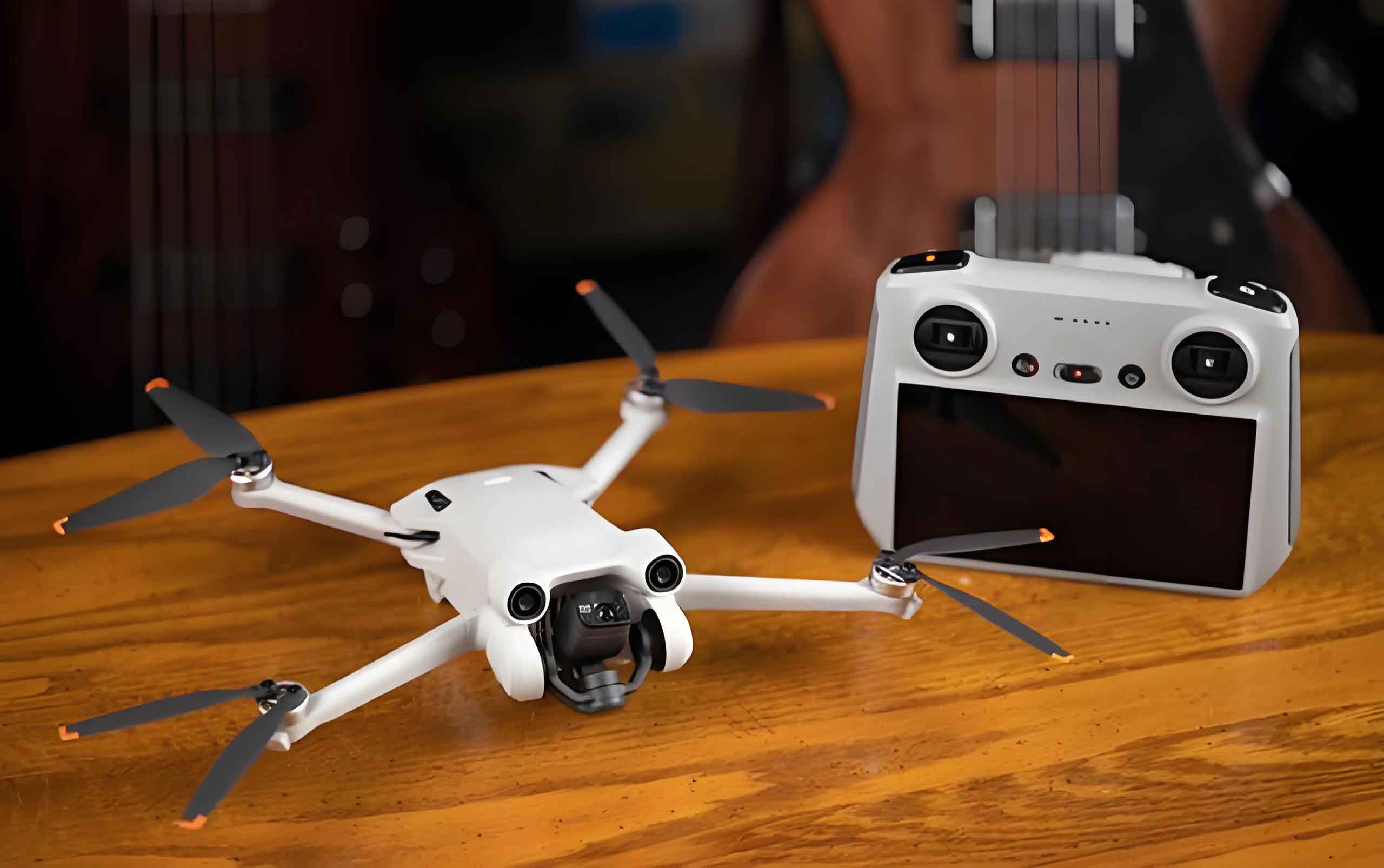
The image above illustrates a typical drone platform equipped with a LiDAR sensor, highlighting the compact design that enables operations in confined spaces. The integration of GNSS antennas (front and back) and the IMU (internal) is critical for the direct georeferencing accuracy discussed earlier.
Environmental Adaptability of Drone Technology
Robustness to Weather Conditions
Traditional aerial photogrammetry relies on sunlight and cloud-free conditions to produce sharp images with sufficient contrast. In contrast, drone LiDAR operates independently of ambient light. We routinely collect data during overcast days, light rain, or even at night. The main weather limitations for drone technology are strong winds (above 10–12 m/s) that destabilize the platform, and heavy precipitation that can scatter laser pulses. Systematic trials have shown that under light drizzle, the point cloud quality degrades by less than 10% in terms of noise, while photogrammetric flights would be completely unfeasible.
Spatial Adaptability
Drone technology enables operations in both open and confined spaces by adjusting flight modes. For instance, in an open field, we use a standard lawnmower pattern at 100 m altitude covering a 500 m swath. In a narrow gorge, we switch to a terrain-following flight at 30 m altitude with a 20° scan angle, ensuring the laser hits the canyon walls vertically. The versatility of the drone platform means that we can produce high-precision DEMs for areas that were previously unmapped due to access constraints.
Key Workflow and Optimization Strategies for High-Precision DEM with Drone LiDAR
Data Acquisition Phase
Precision Flight Planning
Every successful high-precision DEM project begins with meticulous flight planning. We define the required point density based on the desired DEM grid size (e.g., 0.5 m grid demands at least 4 points per cell). Using mission planning software, we set:
- Flight altitude: Determines swath width and point density. For 10 cm DEM, we typically fly at 80–120 m AGL.
- Line spacing and overlap: We maintain at least 80% forward overlap and 60% side overlap to ensure strip registration robustness.
- Terrain awareness: In hilly terrain, we load a coarse existing DEM into the autopilot to adjust altitude dynamically.
An optimized flight plan can reduce redundant data by 20% while guaranteeing coverage.
Equipment Calibration
Before each mission, we perform a boresight calibration flight over a known flat area. The calibration estimates the angular misalignment (roll, pitch, yaw) between the LiDAR sensor and the IMU. This misalignment, if uncorrected, introduces systematic elevation errors up to several centimeters. The calibration procedure solves for three angles \( \delta\phi, \delta\theta, \delta\psi \) by minimizing the discrepancy between overlapping strips:
$$
\min_{\delta\phi,\delta\theta,\delta\psi} \sum_{i=1}^{N} \left( z_{\text{strip1}, i} – z_{\text{strip2}, i} \right)^2
$$
We also verify the GNSS antenna offset and the IMU lever arm. Drone technology streamlines this calibration because we can fly a dedicated 10-minute pattern on site, immediately verifying the corrections.
Ground Control Point Deployment
Although drone LiDAR can achieve good accuracy without ground control points (GCPs) when using PPK/RTK, we typically deploy a small set of GCPs for independent quality control. The GCPs are evenly distributed across the survey area, with extra points near terrain breaks. Each GCP is surveyed with a geodetic-grade GNSS receiver achieving 2 cm accuracy. The following table lists a typical GCP configuration for a 10 km² project:
| GCP Type | Number of Points | Purpose |
|---|---|---|
| Primary GCPs (used for boresight refinement) | 5–8 | Improve absolute horizontal and vertical accuracy |
| Check points (independent verification) | 10–15 | Compute external RMSE of the final DEM |
| Validation points (complex terrain) | 5–10 | Assess fidelity in steep slopes or vegetated zones |
The use of GCPs remains an effective safety net, especially when GNSS conditions are suboptimal (e.g., near high-voltage lines or in deep canyons).
Data Processing Core Steps
Point Cloud Preprocessing
The raw point cloud from drone technology contains noise, outliers, and non-ground points. Preprocessing involves three main steps:
- Statistical outlier removal: Points with Z-values more than 3 standard deviations from the local mean are removed.
- Ground classification: We use an adaptive triangulated irregular network (TIN) densification algorithm. The algorithm starts with the lowest points in a grid, constructs a TIN, and iteratively adds points that lie within a threshold \( d \) from the TIN surface. The threshold increases with slope.
- Coordinate transformation: Raw points are transformed from WGS84 to the local projection (e.g., UTM) using rigorous geodetic formulas.
The quality of classification is critical for DEM accuracy. We typically achieve 95–98% classification accuracy in forested areas using multi-return information (e.g., only the last return is considered ground if the first return has a large vertical gap).
DEM Grid Generation
After extracting ground points, we interpolate them onto a regular grid. The choice of interpolation method affects the DEM‘s smoothness and ability to preserve sharp features. The two most common methods in drone technology workflows are:
- Inverse distance weighting (IDW):
$$
Z(x,y) = \frac{\sum_{i=1}^{n} w_i z_i}{\sum_{i=1}^{n} w_i}, \quad w_i = \frac{1}{d_i^p}
$$
where \( d_i \) is the horizontal distance from the grid cell center to the i-th point, and \( p \) is the power parameter (typically 2). IDW is fast and produces smooth surfaces but may oversmooth sharp edges.
- Kriging (ordinary kriging): Uses a semivariogram model to estimate spatial correlation. While more accurate, it requires careful parameter tuning and is computationally heavier.
For high-precision DEMs, we often employ a hybrid approach: first, we generate a coarse grid using kriging to estimate the overall trend, then we “nudge” the grid points using a localized IDW or natural neighbor method to preserve subtle terrain features. The grid cell size \( \Delta \) is chosen such that:
$$
\Delta \approx \frac{1}{\sqrt{\rho}} \quad \text{or smaller}
$$
ensuring each grid cell contains at least one ground point. For a point density of 25 pt/m², a 0.2 m grid is appropriate.
Edge and Detail Optimization
Boundary areas and zones with rapid elevation change (e.g., cliff edges, river banks) often suffer from artifacts. We apply a specialized “breakline” processing step: we manually or automatically digitize breaklines from the point cloud (using intensity or slope changes) and then enforce these lines as constraints during interpolation. Additionally, we fill small data voids (e.g., due to water absorption) using a spline interpolation guided by surrounding terrain. The final DEM is then smoothed with a low-pass filter (e.g., median filter of 3×3 cells) to remove speckle noise without degrading real terrain edges.
Accuracy Control and Quality Improvement
Multi-Level Accuracy Assessment
We implement a dual verification system: internal consistency checks and external validation. Internal checks compare overlapping strips after boresight correction; the standard deviation of height differences between strips should be less than 3 cm for high-precision work. External validation uses the independent check points (not used in processing) to compute the root mean square error (RMSE):
$$
RMSE_z = \sqrt{\frac{1}{N} \sum_{i=1}^{N} (Z_{\text{DEM},i} – Z_{\text{GCP},i})^2 }
$$
Typical results from our projects using drone technology show RMSE values between 5 and 8 cm for flat terrain and 8–12 cm for steep, forested terrain. The table below summarizes accuracy statistics from three representative projects:
| Project Type | Area (km²) | Terrain Character | Point Density (pt/m²) | RMSE_z (cm) | Max Error (cm) |
|---|---|---|---|---|---|
| Coastal wetland | 3.2 | Flat with channels | 45 | 4.2 | 11.3 |
| Mountainous forest | 8.5 | Steep slopes, 70% tree cover | 28 | 9.8 | 23.5 |
| Urban construction site | 1.7 | Mixed buildings and bare ground | 60 | 3.5 | 8.1 |
These results demonstrate the consistent performance of drone technology across varied environments.
Error Mitigation Strategies
When validation reveals errors beyond acceptable thresholds, we apply targeted corrections:
- Systematic vertical bias: If the entire DEM is shifted by a constant, we apply a uniform correction based on the mean difference between check points and DEM values.
- Strip misalignment: We re-run the strip adjustment algorithm, sometimes adding a few more tie points manually in areas with weak geometry.
- Local point cloud anomalies: For isolated error spikes (e.g., caused by a bird or a low-flying aircraft), we delete the offending points and re-interpolate locally.
- Vegetation penetration failures: In dense undergrowth, we may increase the ‘ground offset‘ parameter in the classification algorithm or use a full-waveform analysis to better separate ground from low vegetation.
Drone technology allows us to seamlessly re-fly small problematic areas within the same mission day, a luxury not available with manned aircraft.
Quality Evaluation Standards
We adopt the following quality metrics for final DEM delivery:
- Vertical accuracy: RMSE ≤ 10 cm for 1:1000 scale mapping; ≤ 5 cm for engineering design.
- Completeness: No data gaps larger than 1 grid cell; voids filled by interpolation with documented method.
- Terrain fidelity: Slope comparison between DEM and independently measured profiles should show correlation > 0.95.
- Artifact detection: No artificial steps, pits, or humps exceeding 2× the expected noise level.
We document all processing steps, calibration values, and accuracy statistics in a metadata report, ensuring traceability and reusability of the DEM product.
Conclusion
Drone technology, when integrated with LiDAR, has revolutionized the production of high-precision DEMs. The direct ranging capability, combined with the flexibility of unmanned platforms, enables us to capture accurate terrain data over large areas in a fraction of the time required by traditional methods. Through rigorous flight planning, equipment calibration, and multi-step data processing, we routinely achieve centimeter-level elevation accuracy even in challenging environments such as dense forests and steep slopes. The systematic use of ground control points, multi-level accuracy assessment, and error correction strategies ensures that the final DEM meets the strictest industry standards. As drone technology continues to advance—with lighter sensors, longer endurance, and improved onboard processing—the potential for even higher resolution and faster turnaround times is immense. I am confident that drone-based LiDAR will become the default method for high-quality DEM generation in the coming years, supporting everything from flood modeling to precision agriculture with unprecedented detail.