
The coordination of multiple unmanned aerial vehicles (UAVs) into precise, dynamic formations represents a significant challenge in control systems engineering. A quintessential and publicly visible application of this technology is the formation drone light show, where hundreds or thousands of drones act as luminous pixels in the night sky. The core technical enabler of such spectacular displays is safe, reliable, and real-time trajectory planning. Each drone must navigate from its starting position to a defined point in a complex, time-varying formation while strictly avoiding collisions with neighboring drones and any static or dynamic obstacles. This paper addresses this critical problem by designing a multi-constrained trajectory planning strategy based on Distributed Model Predictive Control (DMPC). The strategy enables a fleet of drones to generate optimal trajectories from initial positions to target destinations within a predefined formation pattern, all while adhering to state constraints, inter-agent collision avoidance, and obstacle evasion requirements. We begin by establishing a linear time-invariant model for the drone formation’s translational motion. Subsequently, we formulate a DMPC-based optimization problem that incorporates formation-keeping objectives via a consensus-based strategy alongside the aforementioned constraints. The efficacy of the proposed planning algorithm, particularly a novel on-demand collision avoidance method, is validated through numerical simulations against existing benchmarks. Finally, the practical viability of the entire framework is demonstrated via real-world flight experiments using a custom-built multi-drone system operating in a complex, obstacle-laden environment.
The allure of a synchronized formation drone light show lies in its perfect harmony, but this harmony is underpinned by immense computational and control complexity. The primary challenge is to plan and execute smooth, kinematically feasible trajectories for a large number of agents in a shared, potentially cluttered, airspace. Centralized planning methods, which compute trajectories for all agents on a single powerful computer, suffer from scalability issues; the computational cost grows prohibitively with the size of the fleet. Furthermore, they present a single point of failure. Distributed approaches, where each drone computes its own trajectory based on local information, offer a more scalable and robust solution, aligning well with the decentralized nature of a large-scale formation drone light show.
Among distributed methods, Model Predictive Control (MPC) is particularly well-suited. MPC’s core principle is to solve, at each time step, a finite-horizon optimal control problem based on the current state. Only the first control input of the optimized sequence is applied, and the process repeats at the next time step in a “receding horizon” fashion. This allows for:
- Explicit Constraint Handling: Safety constraints like collision avoidance can be directly incorporated into the optimization problem.
- Optimality: The controller naturally trades off competing objectives (e.g., reaching a target vs. saving energy).
- Feedback & Robustness: The repeated re-planning accounts for model inaccuracies and disturbances.
Distributed MPC (DMPC) extends this paradigm by having each agent solve its own local MPC problem. These local problems are coupled through constraints or objectives that depend on the predicted states of neighboring agents, requiring an iterative or coordinated solution process to achieve global coherence—a necessity for a flawless formation drone light show.
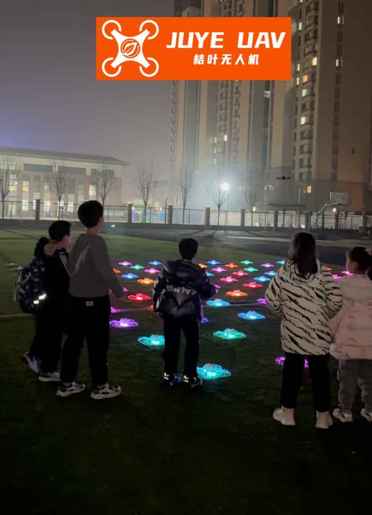
The visual spectacle of a formation drone light show is ultimately a trajectory tracking problem. To cast it into a solvable optimization framework, we first require a mathematical model of the drone’s motion. For trajectory planning purposes, especially in large formations where computational efficiency is paramount, we often simplify the full nonlinear dynamics. We focus on the translational motion in a 3D inertial frame, treating each drone as a point mass with double-integrator dynamics. This captures the essential relationship between commanded acceleration and resulting position.
Let $i \in \{1, 2, …, N\}$ denote the index of a drone in a formation of size $N$. Its kinematic state at continuous time $t$ is defined by its position $\mathbf{p}_i(t) = [x_i(t), y_i(t), z_i(t)]^T \in \mathbb{R}^3$ and its velocity $\mathbf{v}_i(t) = [\dot{x}_i(t), \dot{y}_i(t), \dot{z}_i(t)]^T \in \mathbb{R}^3$. The control input is the acceleration $\mathbf{a}_i(t) \in \mathbb{R}^3$. The continuous-time model is:
$$
\begin{align}
\dot{\mathbf{p}}_i(t) &= \mathbf{v}_i(t), \\
\dot{\mathbf{v}}_i(t) &= \mathbf{a}_i(t).
\end{align}
$$
For digital implementation in MPC, we discretize this model with a sampling period $h$. The discrete-time linear time-invariant (LTI) state-space model for drone $i$ at time step $k$ is:
$$
\mathbf{x}_i[k+1] = \mathbf{A}_i \mathbf{x}_i[k] + \mathbf{B}_i \mathbf{u}_i[k],
$$
where $\mathbf{x}_i[k] = [\mathbf{p}_i[k]^T, \mathbf{v}_i[k]^T]^T \in \mathbb{R}^6$ is the state vector, $\mathbf{u}_i[k] = \mathbf{a}_i[k] \in \mathbb{R}^3$ is the control input (acceleration), and the matrices are:
$$
\mathbf{A}_i =
\begin{bmatrix}
\mathbf{I}_3 & h\mathbf{I}_3 \\
\mathbf{0}_3 & \mathbf{I}_3
\end{bmatrix}, \quad
\mathbf{B}_i =
\begin{bmatrix}
\frac{h^2}{2}\mathbf{I}_3 \\
h\mathbf{I}_3
\end{bmatrix}.
$$
Here, $\mathbf{I}_3$ and $\mathbf{0}_3$ are the $3 \times 3$ identity and zero matrices, respectively.
Communication within the fleet is crucial for distributed coordination. The interaction topology is represented by a graph $\mathcal{G} = (\mathcal{V}, \mathcal{E})$, where $\mathcal{V}$ is the set of $N$ nodes (drones) and $\mathcal{E} \subseteq \mathcal{V} \times \mathcal{V}$ is the set of edges. An edge $(j, i) \in \mathcal{E}$ indicates that drone $i$ can receive state information from drone $j$. The set of neighbors of drone $i$ is $\mathcal{N}_i = \{ j \in \mathcal{V} \setminus \{i\} : (j, i) \in \mathcal{E} \}$. For a formation drone light show, this graph is typically pre-defined and connected to ensure the propagation of formation information.
The core objective is to design a DMPC-based planner that enables the drone fleet to fulfill the following mission:
Given: A fleet of $N$ drones with the model above, an operating workspace $\mathcal{W} \subset \mathbb{R}^3$, and a set of desired final target positions $\mathbf{p}_{d,i} \in \mathcal{W}$.
Generate: For each drone $i$, a sequence of control inputs $\mathbf{u}_i$ that drives it from its initial state $\mathbf{x}_i(0)$ to its target, subject to the following constraints and objectives:
- Target Convergence: $\lim_{t \to \infty} (\mathbf{p}_i(t) – \mathbf{p}_{d,i}) = 0$.
- Formation Keeping: During transit, maintain a desired geometric configuration relative to neighbors: $\lim_{t \to \infty} (\mathbf{p}_j(t) – \mathbf{p}_i(t)) = \mathbf{d}_{ij,ref}$ for all $j \in \mathcal{N}_i$, where $\mathbf{d}_{ij,ref}$ is the desired relative position vector.
- Inter-Agent Collision Avoidance: Maintain a minimum safe distance $r_{min}$ from all other drones: $\| \mathbf{p}_j(t) – \mathbf{p}_i(t) \| \geq r_{min}, \quad \forall j \neq i, \forall t$.
- Obstacle Avoidance: Maintain a minimum safe distance $r_{obs}$ from all static and dynamic obstacles: $\| \mathbf{p}_o(t) – \mathbf{p}_i(t) \| \geq r_{obs}, \quad \forall o \in \mathcal{N}_o, \forall t$, where $\mathcal{N}_o$ is the set of obstacles.
- State and Input Constraints: Respect physical limits: $\mathbf{p}_{min} \leq \mathbf{p}_i \leq \mathbf{p}_{max}$, $\mathbf{v}_{min} \leq \mathbf{v}_i \leq \mathbf{v}_{max}$, $\mathbf{a}_{min} \leq \mathbf{a}_i \leq \mathbf{a}_{max}$.
The DMPC controller works in a receding horizon manner. At each discrete time step $k_t$, corresponding to continuous time $t_0$, drone $i$ solves an optimization problem over a future prediction horizon of $K$ steps (covering time $t \in [t_0, t_0 + T_h]$, $T_h = K \cdot h$). To ensure smoothness and dynamic feasibility of the resulting trajectory, we parameterize the predicted continuous-time position $\mathbf{p}_i(t)$ as a concatenation of $l$ B-spline curves.
A B-spline curve of order $k$ in $\mathbb{R}^3$ is defined by a set of control points $\mathcal{P}_i = \{\mathbf{P}_{i,0}, \mathbf{P}_{i,1}, …, \mathbf{P}_{i,n}\}$ and the B-spline basis functions $B_{m,k}(t)$:
$$
\mathbf{p}_i(t) = \sum_{m=0}^{n} \mathbf{P}_{i,m} B_{m,k}(t).
$$
The control points $\mathcal{P}_i$ become the finite set of decision variables optimized by the MPC. The B-spline formulation guarantees $C^{k-2}$ continuity, which is essential for generating jerk-limited, smooth trajectories suitable for real drone dynamics and for a visually pleasing formation drone light show.
Using the discrete LTI model, the predicted state sequence for drone $i$ over the horizon can be written as an affine function of its planned input sequence. Let the stacked vectors be:
$\mathbf{X}_i = [\mathbf{x}_i[1|k_t]^T, …, \mathbf{x}_i[K|k_t]^T]^T$,
$\mathbf{U}_i = [\mathbf{u}_i[0|k_t]^T, …, \mathbf{u}_i[K-1|k_t]^T]^T$,
and $\mathbf{P}_i = [\mathbf{p}_i[1|k_t]^T, …, \mathbf{p}_i[K|k_t]^T]^T$.
We can write:
$$
\mathbf{P}_i = \mathbf{\Gamma}_i \mathbf{x}_i[k_t] + \mathbf{\Lambda}_i \mathbf{U}_i,
$$
where $\mathbf{\Gamma}_i$ and $\mathbf{\Lambda}_i$ are matrices constructed from $\mathbf{A}_i$, $\mathbf{B}_i$, and the selection matrix $\mathbf{\Psi} = [\mathbf{I}_3, \mathbf{0}_3]$ that extracts position from the state vector. This linear relationship is key to formulating a convex (Quadratic Program) optimization problem.
At each time step $k_t$, drone $i$ solves a local Quadratic Programming (QP) problem. The cost function $J_i$ combines several weighted objectives:
$$
J_i(\mathbf{U}_i, \boldsymbol{\alpha}_i) = J_{i, target} + J_{i, formation} + J_{i, input} + J_{i, violation}.
$$
1. Target Convergence Cost: Penalizes the deviation of the predicted terminal positions from the desired target $\mathbf{p}_{d,i}$. We focus on the last $\theta \leq K$ steps of the horizon to encourage progress.
$$
J_{i, target} = \sum_{k=K-\theta}^{K-1} q_k \| \mathbf{p}_i[k|k_t] – \mathbf{p}_{d,i} \|^2.
$$
This can be written as a quadratic in $\mathbf{U}_i$ using the affine prediction model: $J_{i, target} = \mathbf{U}_i^T \mathbf{H}_t \mathbf{U}_i + \mathbf{f}_t^T \mathbf{U}_i + const.$
2. Formation Keeping Cost: Enforces the desired geometric shape of the formation drone light show. It penalizes deviations from the desired relative positions with respect to neighboring drones $j \in \mathcal{N}_i$.
$$
J_{i, formation} = \sum_{j \in \mathcal{N}_i} \sum_{k=0}^{K-1} q_f \| \mathbf{p}_i[k|k_t] – \mathbf{p}_j[k|k_t] – \mathbf{d}_{ij,ref} \|^2.
$$
This term couples the optimizations of different drones. In the DMPC scheme, drone $i$ uses the most recently communicated assumed trajectory $\tilde{\mathbf{P}}_j$ from its neighbors to evaluate this cost, leading to a quadratic form: $J_{i, formation} = \mathbf{U}_i^T \mathbf{H}_f \mathbf{U}_i + \mathbf{f}_f^T \mathbf{U}_i + const.$
3. Input Smoothing Cost: Penalizes changes in acceleration (jerk) to generate smooth trajectories, reduce actuator wear, and improve passenger comfort in other applications. For a formation drone light show, smoothness is critical for visual quality.
$$
J_{i, input} = \sum_{k=0}^{K-1} q_{\Delta} \| \mathbf{u}_i[k|k_t] – \mathbf{u}_i[k-1|k_t] \|^2.
$$
This is also a quadratic in $\mathbf{U}_i$.
4. Constraint Violation Cost: A penalty on slack variables $\boldsymbol{\alpha}_i$ introduced to soften collision constraints, ensuring the optimization problem remains feasible even in highly constrained scenarios.
$$
J_{i, violation} = \zeta \| \boldsymbol{\alpha}_i \|^2 + \boldsymbol{\xi}^T \boldsymbol{\alpha}_i.
$$
The constraints define the feasible set for the optimization variable $\mathbf{z}_i = [\mathbf{U}_i^T, \boldsymbol{\alpha}_i^T]^T$.
1. Dynamics & Continuity Constraints: The B-spline parameterization inherently enforces continuity. This translates to linear equality constraints on the control points, which in turn are linear in $\mathbf{U}_i$: $\mathbf{A}_{eq} \mathbf{U}_i = \mathbf{b}_{eq}$.
2. State and Input Limits (Physical Constraints): These are box constraints on velocity, acceleration, and workspace boundaries. Using the prediction model $\mathbf{P}_i = \mathbf{\Gamma}_i \mathbf{x}_i[k_t] + \mathbf{\Lambda}_i \mathbf{U}_i$, they become linear inequality constraints:
$$
\mathbf{U}_{min} \leq \mathbf{U}_i \leq \mathbf{U}_{max}, \\
\mathbf{P}_{min} \leq \mathbf{\Gamma}_i \mathbf{x}_i[k_t] + \mathbf{\Lambda}_i \mathbf{U}_i \leq \mathbf{P}_{max}.
$$
3. Collision Avoidance Constraints (The Key Innovation): Enforcing $\| \mathbf{p}_j – \mathbf{p}_i \| \geq r_{min}$ directly leads to non-convex constraints. We employ an on-demand soft-constraint method. At time $k_t$, drone $i$ checks its predicted trajectory (based on its previous plan) against the assumed trajectories of neighbors for potential collisions within the horizon. If a collision with agent $j$ is predicted at step $k_c$, a single linearized avoidance constraint is added only for that specific conflict at the step before collision ($k_c – 1$). The constraint is linearized using the relative position from the previous plan and includes a slack variable $\alpha_{ij} \leq 0$:
$$
\omega_{ij}^T \mathbf{p}_i[k_c – 1|k_t] – \alpha_{ij} \sigma_{ij} \geq \upsilon_{ij},
$$
where $\omega_{ij}$, $\sigma_{ij}$, and $\upsilon_{ij}$ are computed from previous predictions. This “on-demand” approach is more efficient than methods like Buffered Voronoi Cells (BVC) which add constraints at every step, leading to a simpler, sparser, and faster-to-solve QP. This efficiency is paramount for scaling to the size of a major formation drone light show. The set of all such constraints for threatening neighbors $j \in \Delta_i$ forms $\mathbf{A}_{coll} \mathbf{U}_i – \mathbf{S} \boldsymbol{\alpha}_i \leq \mathbf{b}_{coll}$.
4. Obstacle Avoidance: Static and dynamic obstacles are treated similarly. For a spherical obstacle $o$ with center $\mathbf{p}_o$, a constraint $\| \mathbf{p}_i – \mathbf{p}_o \| \geq r_{obs}$ is linearized and added on-demand if a violation is predicted.
The complete local QP for drone $i$ at time $k_t$ is:
$$
\begin{aligned}
\min_{\mathbf{z}_i} \quad & \frac{1}{2} \mathbf{z}_i^T \mathbf{H}_i \mathbf{z}_i + \mathbf{f}_i^T \mathbf{z}_i \\
\text{subject to} \quad & \mathbf{A}_{eq} \mathbf{U}_i = \mathbf{b}_{eq}, \\
& \mathbf{A}_{in} \mathbf{U}_i \leq \mathbf{b}_{in}, \\
& \mathbf{A}_{coll} \mathbf{U}_i – \mathbf{S} \boldsymbol{\alpha}_i \leq \mathbf{b}_{coll}, \\
& \boldsymbol{\alpha}_i \leq \mathbf{0}.
\end{aligned}
$$
Where $\mathbf{H}_i$ and $\mathbf{f}_i$ aggregate the quadratic and linear cost terms from $J_i$. All drones solve their QPs in parallel after exchanging their latest assumed trajectories. This parallel, distributed solution is the cornerstone of real-time planning for a formation drone light show.
The performance of the proposed DMPC planner with on-demand collision avoidance was first validated in high-fidelity numerical simulations. A scenario with $N=4$ drones and multiple static/dynamic obstacles was constructed. The drones were tasked with navigating to their targets while forming and maintaining a square formation. Key metrics were tracked.
Formation Performance: The formation error $\chi(k) = \sum_{i=1}^N \sum_{j \in \mathcal{N}_i} (\| \mathbf{p}_j(k) – \mathbf{p}_i(k) \| – \| \mathbf{d}_{ij,ref} \|)^2$ rapidly converged to near zero upon formation assembly. During obstacle avoidance maneuvers, the error increased slightly as the formation flexed, but it quickly recovered afterward, demonstrating the algorithm’s ability to maintain cohesive flight for a formation drone light show even under duress.
Safety: The minimum inter-agent distance and the minimum agent-obstacle distance remained strictly above the safety thresholds ($r_{min}=0.2m$, $r_{obs}=0.2m$) at all times.
Computational Efficiency: The average QP solution time per drone per time step was under 4 milliseconds on a standard desktop CPU. This leaves ample margin for communication and other onboard processes, confirming real-time feasibility.
A critical comparative analysis was conducted against the established Buffered Voronoi Cell (BVC) method. The same simulation scenario was run with BVC-based collision constraints replacing the on-demand method. The results are summarized below:
| Performance Metric | Proposed On-Demand Method | BVC Method |
|---|---|---|
| Average Trajectory Length per Drone | 21.3 m | 22.0 m |
| Average Flight Speed | 0.77 m/s | 0.72 m/s |
| Average Solving Time (per drone per step) | 3.94 ms | 12.91 ms |
| Total Mission Time | 27.66 s | 30.65 s |
The on-demand method outperformed BVC in all key metrics: it generated shorter, faster trajectories (indicating better optimality), completed the mission quicker, and—most importantly—solved the local QP more than three times faster. This dramatic reduction in computation time is a direct result of adding constraints only when necessary, rather than conservatively at every step. This efficiency gain is a decisive advantage for scaling up to the hundreds of agents in a large formation drone light show.
To bridge the gap between simulation and reality, the DMPC algorithm was implemented on a custom fleet of quadcopter drones. The experimental setup consisted of 3 formation drones and 1 drone acting as a dynamic obstacle. An OptiTrack motion capture system provided precise, real-time pose data for all agents. Each drone was equipped with an onboard computer (Nvidia Jetson) running the local DMPC planner at 20 Hz. The planners received state information via a WiFi network and sent computed acceleration commands to a Pixhawk flight controller running a low-level attitude stabilizer.
The mission involved the 3 formation drones starting from dispersed locations, navigating through a space containing static poles (cylindrical obstacles) and a moving obstacle drone, to reach their target positions while forming a triangle. The dynamic obstacle followed a pre-defined path intersecting the formation’s intended flight path.
Experimental Results: The fleet successfully executed the mission. The recorded trajectories showed smooth, coordinated motion. Crucially, the minimum recorded distances confirmed safety: inter-drone distances stayed above 0.4m and drone-obstacle distances stayed above 0.5m, respecting the defined safety margins with added buffer for real-world uncertainty. The formation error remained low throughout the flight, spiking only momentarily during the close encounter with the dynamic obstacle before rapidly re-converging. This experiment tangibly proves that the proposed DMPC framework can generate safe, cooperative, and real-time trajectories for physical drones, a fundamental requirement for deploying an outdoor formation drone light show.
This work presented a comprehensive DMPC-based trajectory planning framework for multi-drone formations, with a focus on the demanding application of a formation drone light show. The contributions are multifold: a formulation that integrates target reaching, formation keeping, and multi-agent/obstacle avoidance into a single optimization problem; the development of an efficient on-demand collision constraint method that significantly reduces computational load compared to state-of-the-art approaches like BVC; and the validation of the entire pipeline through both high-fidelity simulation and real-world flight experiments.
The results consistently demonstrate that the algorithm ensures safety (no collisions), maintains formation cohesion, respects physical limits, and operates in real-time on embedded hardware. The parallelizable nature of the distributed solution makes it highly scalable. Future work will focus on incorporating more detailed vehicle dynamics, explicitly accounting for aerodynamic downwash between closely packed drones in a formation drone light show, and extending the framework to handle partial communication loss and more complex, unstructured outdoor environments. The path towards ever more ambitious and reliable aerial displays is paved by such advances in robust, distributed control theory.