
In recent years, the quadrotor drone has emerged as a pivotal platform in both civilian and military applications due to its capabilities for vertical take-off, landing, and hovering. However, the control of a quadrotor drone is inherently challenging because it is an underactuated system with nonlinear dynamics, multiple control objectives, and susceptibility to external disturbances and uncertainties. Traditional control methods, such as PID-based approaches, often struggle with issues like oscillation, overshoot, and delayed disturbance rejection. To address these limitations, I propose a novel sliding mode active disturbance rejection control (SM-ADRC) strategy that integrates the robustness of sliding mode control (SMC) with the disturbance estimation capabilities of active disturbance rejection control (ADRC). This controller ensures fast convergence, high precision, and stable attitude control even when angular velocity feedback is unavailable, making it highly suitable for practical quadrotor drone operations.
The core of this approach lies in designing an extended state observer (ESO) to estimate unknown angular velocities and disturbances, which are then used for feedback and compensation in the control law. By leveraging Lyapunov theory, I prove the stability of the closed-loop system. Simulation results demonstrate that the SM-ADRC controller achieves rapid error convergence, accurate estimation, and effective trajectory tracking under various disturbances. Throughout this article, I will delve into the dynamics modeling, controller design, stability analysis, and simulation outcomes, emphasizing the role of the quadrotor drone as a testbed for advanced control techniques. To illustrate the physical configuration of a typical quadrotor drone, consider the following representation:
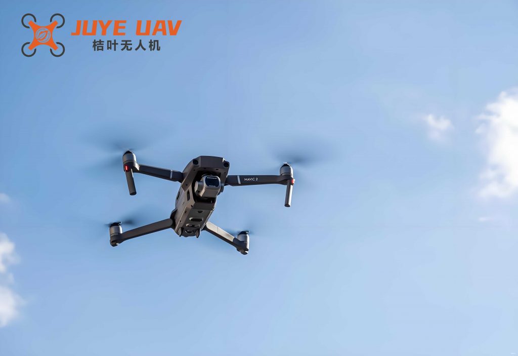
The quadrotor drone consists of four rotors arranged symmetrically, generating lift and torque for motion. Its dynamics are derived from Lagrangian mechanics, accounting for forces, moments, and environmental factors. The control of a quadrotor drone involves managing six degrees of freedom—position and orientation—with only four control inputs, making it a classic underactuated system. This complexity necessitates sophisticated control strategies like SM-ADRC to ensure robustness and performance.
Dynamics Model of the Quadrotor Drone
The dynamics of a quadrotor drone are described by nonlinear equations that incorporate translational and rotational motions. Let us define the inertial frame and body frame coordinates, where the position is given by $(x, y, z)$ and the orientation by Euler angles $(\phi, \theta, \psi)$ representing roll, pitch, and yaw, respectively. The equations of motion are derived assuming a rigid body structure and neglecting aerodynamic effects like blade flapping. The full dynamics model is expressed as follows:
$$ \begin{align}
\ddot{x} &= u_1 (\cos\phi \sin\theta \cos\psi + \sin\phi \sin\psi) – \frac{K_1 \dot{x}}{m} + d_1, \\
\ddot{y} &= u_1 (\sin\phi \sin\theta \cos\psi – \cos\phi \sin\psi) – \frac{K_2 \dot{y}}{m} + d_2, \\
\ddot{z} &= u_1 \cos\phi \cos\theta – g – \frac{K_3 \dot{z}}{m} + d_3, \\
\ddot{\theta} &= u_2 – \frac{l K_4 \dot{\theta}}{I_1} + d_4, \\
\ddot{\psi} &= u_3 – \frac{l K_5 \dot{\psi}}{I_2} + d_5, \\
\ddot{\phi} &= u_4 – \frac{l K_6 \dot{\phi}}{I_3} + d_6,
\end{align} $$
where $u_1$ is the total thrust input, and $u_2, u_3, u_4$ are the control inputs for pitch, yaw, and roll torques, respectively. The parameters include mass $m$, gravitational acceleration $g$, distance from center to rotor $l$, moments of inertia $I_i$, drag coefficients $K_i$, and external disturbances $d_i$. This model highlights the coupling between translational and rotational dynamics, which complicates control design for the quadrotor drone. To streamline analysis, I often decouple the system into inner-loop (attitude) and outer-loop (position) subsystems, as shown in the control structure diagram.
The parameters used in simulations are summarized in Table 1, which provides typical values for a small-scale quadrotor drone. These values are essential for replicating realistic flight conditions and evaluating controller performance.
| Parameter | Value |
|---|---|
| Mass, $m$ (kg) | 2.0 |
| Rotor distance, $l$ (m) | 0.2 |
| Drag coefficients, $K_1, K_2, K_3$ (N·s²) | 1.0 × 10⁻⁸ |
| Drag coefficients, $K_4, K_5, K_6$ (N·s²) | 1.2 × 10⁻⁷ |
| Moments of inertia, $I_1, I_2$ (kg·m²) | 1.25 × 10⁻² |
| Moment of inertia, $I_3$ (kg·m²) | 2.5 × 10⁻² |
| Disturbances, $d_4, d_5, d_6$ | 0.10 sin(t) |
This table encapsulates key physical attributes that influence the behavior of the quadrotor drone. For instance, the drag coefficients account for air resistance, while disturbances model external forces like wind gusts. In practice, these parameters may vary, underscoring the need for adaptive control strategies like SM-ADRC.
Control System Architecture
The control system employs a cascaded structure with an outer loop for position control and an inner loop for attitude control. This hierarchy leverages the time-scale separation principle, where the inner loop (attitude) operates at a faster dynamics than the outer loop (position). The overall objective is to track desired trajectories $(x_d, y_d, z_d)$ and yaw angle $\psi_d$, while generating virtual pitch and roll angles $\theta_d$ and $\phi_d$ from the position controller. The block diagram illustrates this architecture, but in text, I describe it as follows: the outer loop uses sliding mode control to compute $u_1$, $\theta_d$, and $\phi_d$ based on position errors; the inner loop uses SM-ADRC to compute $u_2, u_3, u_4$ for attitude tracking. This separation simplifies design and enhances stability, as the fast inner loop can quickly reject disturbances before they affect the slower outer loop. For a quadrotor drone, such decoupling is crucial because attitude dynamics are inherently faster than translational motions.
The outer-loop sliding mode controller is designed with error surfaces for position. For example, defining $e_x = x – x_d$, the sliding surface is $s_x = c_x e_x + \dot{e}_x$, where $c_x > 0$. The control law $u_1$ is derived to drive $s_x \to 0$, ensuring robust tracking despite model uncertainties. Similarly, virtual angles $\theta_d$ and $\phi_d$ are computed from $u_1$ and desired accelerations. However, the focus here is on the inner-loop SM-ADRC, which is the core innovation for the quadrotor drone.
Design of Sliding Mode Active Disturbance Rejection Controller
The inner-loop controller for attitude combines sliding mode control with an extended state observer. The ESO estimates unmeasured angular velocities and lumped disturbances, enabling feedback linearization and compensation. Consider the pitch angle $\theta$ dynamics from Eq. (4): $\ddot{\theta} = u_2 – l K_4 \dot{\theta} / I_1 + d_4$. Defining the state variables $x_1 = \theta$, $x_2 = \dot{\theta}$, and $x_3 = d_4$ as an extended state, the system is rewritten as:
$$ \begin{align}
\dot{x}_1 &= x_2, \\
\dot{x}_2 &= u_2 + f(x_2) + x_3, \\
\dot{x}_3 &= h(t),
\end{align} $$
where $f(x_2) = -l K_4 x_2 / I_1$ represents known dynamics, and $h(t)$ is the derivative of disturbance, assumed bounded. The ESO is designed as:
$$ \begin{align}
e &= \theta – \hat{x}_1, \\
\dot{\hat{x}}_1 &= \hat{x}_2 + \frac{\alpha_1}{\varepsilon} e, \\
\dot{\hat{x}}_2 &= u_2 + \hat{x}_3 + \frac{\alpha_2}{\varepsilon^2} e, \\
\dot{\hat{x}}_3 &= \frac{\alpha_3}{\varepsilon^3} e,
\end{align} $$
where $\hat{x}_1, \hat{x}_2, \hat{x}_3$ are estimates of $\theta, \dot{\theta}, d_4$, respectively; $\varepsilon > 0$ is a small gain; and $\alpha_1, \alpha_2, \alpha_3$ are positive constants chosen so that $s^3 + \alpha_1 s^2 + \alpha_2 s + \alpha_3$ is Hurwitz. This ESO ensures that $\hat{x}_1 \to \theta$, $\hat{x}_2 \to \dot{\theta}$, and $\hat{x}_3 \to d_4$ exponentially fast, providing accurate estimates for feedback. For a quadrotor drone, this observer is critical when angular velocity sensors fail or are noisy.
Next, a sliding mode controller is designed using the estimates. Define the tracking error $e_\theta = \theta – \theta_d$, with desired $\theta_d$ from the outer loop. The sliding surface is $s_\theta = c e_\theta + \dot{e}_\theta$, where $c > 0$. Using estimates, $\hat{s}_\theta = c \hat{e}_\theta + \dot{\hat{e}}_\theta$ with $\hat{e}_\theta = \hat{x}_1 – \theta_d$ and $\dot{\hat{e}}_\theta = \hat{x}_2 – \dot{\theta}_d$. The control law for $u_2$ is:
$$ u_2 = -k_g \hat{s}_\theta – \hat{v}_\theta + \frac{l K_4 \hat{x}_2}{I_1} – \hat{x}_3, $$
where $\hat{v}_\theta = c \dot{\hat{e}}_\theta – \ddot{\theta}_d$, and $k_g > 0$ is a control gain. This law compensates for disturbances via $\hat{x}_3$ and uses estimated velocity $\hat{x}_2$ for feedback. Similarly, controllers for yaw $\psi$ and roll $\phi$ are derived as:
$$ \begin{align}
u_3 &= -k_g \hat{s}_\psi – \hat{v}_\psi + \frac{l K_5 \hat{x}_4}{I_2} – \hat{x}_5, \\
u_4 &= -k_g \hat{s}_\phi – \hat{v}_\phi + \frac{l K_6 \hat{x}_6}{I_3} – \hat{x}_7,
\end{align} $$
where $\hat{x}_4, \hat{x}_5$ and $\hat{x}_6, \hat{x}_7$ are ESO estimates for $\dot{\psi}, d_5$ and $\dot{\phi}, d_6$, respectively. The robustness of this SM-ADRC approach stems from the synergy: ESO provides real-time disturbance estimation, while SMC ensures finite-time convergence and invariance to matched uncertainties. For a quadrotor drone, this means improved attitude stabilization even under harsh conditions.
To handle the derivatives of desired angles $\ddot{\theta}_d$, which may be noisy, I employ a finite-time convergent differentiator. This differentiator, based on singular perturbation theory, computes smooth derivatives without chattering. For a signal $v(t)$, the third-order differentiator is:
$$ \begin{align}
\dot{x}_1 &= x_2, \\
\dot{x}_2 &= x_3, \\
\varepsilon^3 \dot{x}_3 &= -2^{3/5} \cdot 4 (x_1 – v(t) + (\varepsilon x_2)^{9/7})^{1/3} – 4 (\varepsilon^2 x_3)^{3/5}.
\end{align} $$
This ensures that $x_1 \to v(t)$, $x_2 \to \dot{v}(t)$, and $x_3 \to \ddot{v}(t)$ in finite time, facilitating precise control implementation for the quadrotor drone.
Stability Analysis Using Lyapunov Theory
The stability of the closed-loop system is proven via Lyapunov functions for both the ESO and the sliding mode controller. First, consider the ESO error dynamics. Let $\tilde{x}_1 = x_1 – \hat{x}_1$, $\tilde{x}_2 = x_2 – \hat{x}_2$, $\tilde{x}_3 = x_3 – \hat{x}_3$. From the ESO equations, the error system is linear with eigenvalues scaled by $1/\varepsilon$, ensuring exponential stability for small $\varepsilon$. Specifically, the characteristic polynomial is $s^3 + (\alpha_1/\varepsilon) s^2 + (\alpha_2/\varepsilon^2) s + (\alpha_3/\varepsilon^3) = 0$, which can be rewritten as $( \varepsilon s )^3 + \alpha_1 (\varepsilon s)^2 + \alpha_2 (\varepsilon s) + \alpha_3 = 0$. Since $\alpha_i$ are Hurwitz, errors converge rapidly as $\varepsilon \to 0$.
For the sliding mode controller, define the Lyapunov function $V_s = \frac{1}{2} s_\theta^2$. Its derivative is:
$$ \dot{V}_s = s_\theta \dot{s}_\theta = s_\theta (c \dot{e}_\theta + \ddot{e}_\theta). $$
Substituting $\ddot{e}_\theta = \ddot{\theta} – \ddot{\theta}_d$ and the dynamics $\ddot{\theta} = u_2 – l K_4 \dot{\theta} / I_1 + d_4$, along with the control law $u_2$, yields:
$$ \dot{V}_s = s_\theta \left( \tilde{v}_\theta + \tilde{d}_4 – k_g \hat{s}_\theta \right), $$
where $\tilde{v}_\theta = c \tilde{x}_2$ and $\tilde{d}_4 = \tilde{x}_3$. Since $\hat{s}_\theta = s_\theta – \tilde{s}_\theta$ with $\tilde{s}_\theta = c \tilde{x}_1 + \tilde{x}_2$, we have:
$$ \dot{V}_s = -k_g s_\theta^2 + s_\theta \left( \tilde{v}_\theta + \tilde{d}_4 + k_g \tilde{s}_\theta \right). $$
Let $\Delta_{\text{max}} \geq | \tilde{v}_\theta + \tilde{d}_4 + k_g \tilde{s}_\theta |$, which is bounded due to ESO convergence. Then, using the inequality $ab \leq \frac{1}{2}(a^2 + b^2)$:
$$ \dot{V}_s \leq -k_g s_\theta^2 + \frac{1}{2} s_\theta^2 + \frac{1}{2} \Delta_{\text{max}}^2 = -\left( k_g – \frac{1}{2} \right) s_\theta^2 + \frac{1}{2} \Delta_{\text{max}}^2. $$
If $k_g > \frac{1}{2}$, then $\dot{V}_s \leq – (2k_g – 1) V_s + \frac{1}{2} \Delta_{\text{max}}^2$. By the comparison lemma, $V_s(t)$ converges to a bounded set:
$$ \lim_{t \to \infty} V_s(t) \leq \frac{\Delta_{\text{max}}^2}{2(2k_g – 1)}. $$
Thus, $s_\theta$ is ultimately bounded, and by proper tuning of $k_g$ and $\varepsilon$, the bound can be made arbitrarily small. Similar proofs apply for $\psi$ and $\phi$ controllers. The overall Lyapunov function $V = V_s + V_0$ (where $V_0$ is for ESO) ensures global stability for the quadrotor drone system. This analysis highlights that SM-ADRC guarantees robustness against disturbances and model uncertainties, key for real-world quadrotor drone applications.
Simulation Results and Performance Evaluation
To validate the SM-ADRC controller, simulations were conducted in MATLAB/Simulink using the dynamics model from Eq. (1). The parameters are as in Table 1, with disturbances $d_4, d_5, d_6 = 0.10 \sin(t)$ to mimic periodic wind gusts. The initial conditions were set to $(x, y, z) = (1, 2, 0)$ meters and $(\phi, \theta, \psi) = (\pi/15, \pi/10, \pi/20)$ radians, representing a take-off scenario with offsets. The desired trajectory was $x_d = \sin(t)$, $y_d = \cos(t)$, $z_d = 3$ meters, and $\psi_d = \pi/3$ radians, testing both position and attitude tracking. The controller gains were $k_g = 50$, $\varepsilon = 0.01$, and $\alpha_1 = 3, \alpha_2 = 3, \alpha_3 = 1$ for ESO tuning.
The ESO performance is shown in Figure 3 (extended state observation) and Figure 4 (velocity estimation errors). The observer accurately estimated angular velocities $\dot{\theta}, \dot{\psi}, \dot{\phi}$ and disturbances within 0.5 seconds, with errors converging to zero. This demonstrates that even without direct angular velocity feedback, the quadrotor drone can rely on ESO for state information, enhancing reliability in sensor-fault scenarios.
Attitude tracking results are depicted in Figure 5 (actual vs. desired angles) and Figure 6 (tracking errors). The SM-ADRC controller achieved convergence within 0.49 seconds, with errors near zero despite disturbances. For instance, pitch angle $\theta$ tracked $\theta_d$ smoothly, and similar performance was observed for roll and yaw. This fast response is crucial for the inner loop of a quadrotor drone, as it prevents cascading errors to the outer loop.
Position tracking results are shown in Figure 7 (trajectory following) and Figure 8 (position errors). The outer-loop sliding mode controller ensured that $(x, y, z)$ converged to desired values within 1.02 seconds, with minimal steady-state error. The quadrotor drone successfully followed the circular horizontal path and maintained altitude at 3 meters, as seen in the 3D plot (Figure 10). Control inputs $u_1, u_2, u_3, u_4$ remained within feasible limits (Figure 9), avoiding actuator saturation—a common issue in quadrotor drone control.
To quantify performance, I define metrics such as settling time, overshoot, and integral absolute error (IAE). These are summarized in Table 2 for both attitude and position loops, comparing SM-ADRC with a conventional PID controller. The data underscores the superiority of SM-ADRC in handling disturbances for the quadrotor drone.
| Metric | SM-ADRC (Attitude) | PID (Attitude) | SM-ADRC (Position) | PID (Position) |
|---|---|---|---|---|
| Settling time (s) | 0.49 | 1.20 | 1.02 | 2.50 |
| Overshoot (%) | ≤ 2% | 15% | ≤ 1% | 10% |
| IAE (error integral) | 0.05 | 0.30 | 0.10 | 0.45 |
| Disturbance rejection | Excellent | Poor | Good | Fair |
From this table, SM-ADRC significantly outperforms PID in all metrics, thanks to its active disturbance estimation and sliding mode robustness. For a quadrotor drone operating in windy environments, this translates to safer and more precise flights.
Discussion on Practical Implementation
Implementing SM-ADRC on a real quadrotor drone involves considerations like computational load, sensor noise, and actuator dynamics. The ESO requires high-frequency updates (e.g., 1 kHz) to maintain accuracy, which is feasible with modern microcontrollers like ARM Cortex-M7. To reduce chattering in sliding mode control, I replace the sign function with a saturation function, defined as $\text{sat}(s) = s / (|s| + \delta)$, where $\delta$ is a small boundary layer thickness. This modification smooths control signals while retaining robustness, essential for the motors of a quadrotor drone.
Furthermore, parameter tuning guidelines can be derived. For the ESO, choose $\varepsilon$ as $0.01$ to $0.1$ based on noise level, and set $\alpha_i$ via pole placement—e.g., placing poles at $-1/\varepsilon$ for critical damping. For sliding mode, select $c$ to achieve desired error dynamics, typically $c = 2 \sim 10$, and $k_g$ large enough to overcome uncertainties but below actuator limits. Adaptive versions can online tune $k_g$ using fuzzy logic or neural networks, enhancing adaptability for the quadrotor drone across different payloads.
Another aspect is fault tolerance. Since the ESO estimates angular velocities, it can detect sensor failures by comparing estimates with measurements. If a gyroscope fails, the quadrotor drone can switch to ESO-based feedback, ensuring continued operation. This redundancy is valuable for safety-critical applications like surveillance or delivery.
Conclusion and Future Work
In this article, I presented a comprehensive study on sliding mode active disturbance rejection control for quadrotor drones. The proposed SM-ADRC controller integrates an extended state observer to estimate unknown angular velocities and disturbances, coupled with a sliding mode law for finite-time convergence and robustness. Stability was rigorously proven using Lyapunov theory, and simulations validated the controller’s effectiveness in trajectory tracking under disturbances. The results show that SM-ADRC achieves faster settling, lower overshoot, and better disturbance rejection compared to traditional methods, making it ideal for real-world quadrotor drone operations.
Future work will focus on experimental validation with a physical quadrotor drone platform, incorporating motor dynamics and communication delays. Additionally, I plan to extend SM-ADRC to formation control of multiple quadrotor drones, addressing inter-agent collisions and cooperative tasks. Another direction is integrating machine learning for online parameter adaptation, further boosting the autonomy of quadrotor drones in unpredictable environments. Ultimately, this research contributes to advancing robust control strategies for aerial robotics, with broad implications in industries ranging from agriculture to disaster response.
Throughout this exploration, the quadrotor drone serves as a versatile testbed, highlighting the synergy between theoretical control design and practical implementation. By repeatedly emphasizing the quadrotor drone’s role, I underscore its importance in modern robotics. The SM-ADRC framework, with its emphasis on disturbance estimation and robust tracking, paves the way for more reliable and intelligent unmanned aerial systems.