
In this work, we present a comprehensive investigation into the application of an improved metaheuristic algorithm for three-dimensional path planning of drone technology. The core contribution of this research is a multi-strategy fusion particle swarm-butterfly optimization improvement algorithm, which we refer to as IPSOBOA. This algorithm is specifically designed to address the inherent challenges of drone technology in complex threat environments, where the path planning problem involves high computational complexity and the difficulty of generating high-quality feasible paths within effective time constraints. Our approach integrates several advanced mechanisms, including Tent chaotic mapping combined with opposition-based learning for population initialization, nonlinear parameter adjustment with dynamic transition probability control, and the incorporation of particle swarm optimization velocity dynamics into the butterfly optimization framework. Through extensive simulation experiments across both static and dynamic environments, we demonstrate that our proposed IPSOBOA significantly outperforms existing algorithms in terms of solution quality, convergence speed, and path safety.
The motivation for this study stems from the rapid proliferation of drone technology across military and civilian applications, including agricultural monitoring, logistics delivery, search and rescue operations, and air traffic management. As drone technology continues to evolve, the operational environments become increasingly complex, characterized by multiple threats such as radar detection zones, no-fly zones, and various static and dynamic obstacles. The path planning problem for drone technology must simultaneously satisfy multiple constraints, including path length minimization, threat avoidance, flight altitude regulation, and trajectory smoothness. Traditional path planning methods often struggle to balance these competing objectives, motivating the development of more sophisticated optimization algorithms. The butterfly optimization algorithm, with its simple structure, few parameters, and strong global search capability, has emerged as a promising candidate for drone technology path planning. However, the standard butterfly optimization algorithm suffers from slow convergence in later iterations and a tendency to become trapped in local optima. Our proposed IPSOBOA addresses these limitations through a series of strategic modifications.
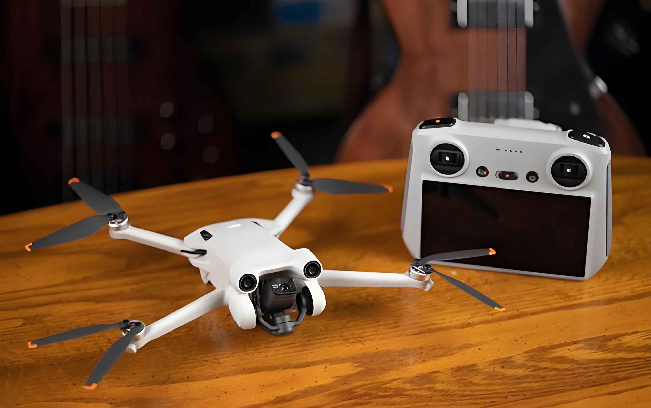
The remainder of this article is organized as follows. We first formulate the path planning problem for drone technology by defining a comprehensive fitness function that incorporates multiple cost components. We then present the detailed design of the IPSOBOA algorithm, including the mathematical formulations of each improvement strategy. Subsequently, we describe the improved dynamic window approach for real-time obstacle avoidance in dynamic environments. Finally, we present extensive experimental results and discuss the implications of our findings for advancing drone technology.
Problem Formulation for Drone Technology Path Planning
The path planning problem for drone technology involves finding an optimal or near-optimal trajectory from a starting point to a target destination while satisfying various operational constraints. In our formulation, each candidate path is represented as a sequence of waypoints, where each waypoint is defined by its three-dimensional coordinates. The quality of a path is evaluated using a multi-objective fitness function that comprises four distinct cost components: path length cost, threat cost, flight altitude cost, and smoothness cost. The overall fitness function is defined as a weighted sum of these components, where lower fitness values indicate superior paths.
Path Length Cost
The path length cost represents the total Euclidean distance traveled by the drone along the candidate path. For a path consisting of consecutive waypoints, the path length cost is calculated as the sum of Euclidean distances between adjacent waypoints. This cost component directly correlates with energy consumption and mission time, making it a primary optimization objective for drone technology applications. The mathematical formulation is given by:
$$F_1(W_i) = \sum_{j=1}^{N-1} \|P_{i,j}P_{i,j+1}\|$$
where represents the complete flight path, denotes the number of waypoints, and is the position vector of the -th waypoint in the -th path. Minimizing this cost ensures that the drone follows the shortest possible route, thereby reducing fuel consumption and mission duration.
Threat Cost
In real-world operational scenarios, drone technology must navigate through environments containing various threats. We consider three types of threats in our model: radar detection zones, no-fly zones, and physical obstacles. Radar threats are modeled as hemispherical regions where the probability of detection increases as the drone approaches the radar center. The radar detection probability is expressed as:
$$P_r(d_r) = \begin{cases} 0, & d_r > R_{\max} \\ \frac{1}{d_r^4}, & R_{\min} \leq d_r \leq R_{\max} \\ 1, & d_r < R_{\min} \end{cases}$$
where represents the distance between the drone and the radar source, is the maximum detection radius, and is the high-risk zone radius. The threat cost associated with radar exposure is computed as:
$$F_i(P_r) = \begin{cases} \infty, & P_r = 1, i \leq N \\ T \cdot P_r, & 0 \leq P_r < 1, i \leq N \end{cases}$$
For obstacles and no-fly zones, we model them as cylindrical regions with defined radii and heights. The drone must maintain a safe distance from these obstacles to avoid collisions. The obstacle threat cost is calculated based on the shortest distance between the path segments and the obstacle centers:
$$T(W_i) = \begin{cases} 0, & d_k > C + D + R_k \\ \sum_{j=1}^{N-1} \sum_{k=1}^{K} (C + D + R_k) – d_k, & D + R_k < d_k \leq C + D + R_k \\ \infty, & d_k \leq D + R_k \end{cases}$$
where represents the diameter of the drone, denotes the safety margin between waypoints, is the radius of the -th obstacle, and is the minimum distance from the -th threat center to the -th path segment. The total threat cost combines both radar and obstacle components:
$$F_2(W_i) = T(W_i) + F_i(P_r)$$
Flight Altitude Cost
Maintaining an appropriate flight altitude is crucial for both safety and efficiency in drone technology operations. The altitude cost encourages the drone to fly at an optimal altitude that balances terrain clearance and energy efficiency. The altitude cost is computed as:
$$F_3(W_i) = \sum_{j=1}^{N} H_{i,j}$$
where the altitude penalty for each waypoint is defined as:
$$H_{i,j} = \begin{cases} \left| h_{i,j} – \frac{h_{\max} + h_{\min}}{2} \right|, & h_{\min} \leq h_{i,j} \leq h_{\max} \\ \infty, & \text{otherwise} \end{cases}$$
Here, represents the altitude of the -th waypoint, while and denote the maximum and minimum allowable flight altitudes, respectively. This formulation penalizes deviations from the optimal cruising altitude while enforcing strict altitude bounds.
Smoothness Cost
The smoothness cost evaluates the maneuverability requirements of the candidate path by considering both turning angles and climbing angles. Smooth paths reduce mechanical stress on the drone structure and improve flight stability, which is particularly important for drone technology applications requiring stable sensor platforms. The turning angle between consecutive path segments is calculated as:
$$\phi_{i,j} = \arctan\left( \frac{\|P’_{i,j}P’_{i,j+1} \times P’_{i,j+1}P’_{i,j+2}\|}{P’_{i,j}P’_{i,j+1} \cdot P’_{i,j+1}P’_{i,j+2}} \right)$$
The climbing angle is computed as:
$$\theta_{i,j} = \arctan\left( \frac{z_{i,j+1} – z_{i,j}}{\|P’_{i,j}P’_{i,j+1}\|} \right)$$
The smoothness cost is then expressed as:
$$F_4(W_i) = \sum_{j=1}^{N-2} (a_1\phi_{i,j} + a_2|\theta_{i,j+1} – \theta_{i,j}|)$$
where and are penalty coefficients for turning and climbing angles, respectively. The overall fitness function that integrates all four cost components is:
$$F(W_i) = \sum_{k=1}^{4} c_k F_k(W_i)$$
where represents the weight coefficient for the -th cost component. These weights are tuned to reflect the relative importance of each objective in the specific drone technology mission context.
The IPSOBOA Algorithm for Drone Technology
The butterfly optimization algorithm is inspired by the foraging and mating behaviors of butterflies in nature. In the standard algorithm, each butterfly emits a fragrance that is perceived by other butterflies, enabling communication and collective movement toward optimal solutions. The fragrance intensity is modulated by a power exponent and a sensory modality parameter. Despite its effectiveness in many optimization problems, the standard butterfly optimization algorithm exhibits limitations when applied to complex drone technology path planning problems, particularly in terms of premature convergence and insufficient exploration capability.
Tent Chaotic Mapping with Opposition-Based Learning
To enhance the diversity of the initial butterfly population and ensure uniform coverage of the search space, we employ a Tent chaotic mapping combined with opposition-based learning for population initialization. The Tent chaotic mapping generates sequences with superior uniformity compared to other chaotic mappings such as the Logistic mapping. The improved Tent chaotic mapping is mathematically expressed as:
$$x_{i+1} = \begin{cases} 2x_i + \frac{\text{rand}(0,1)}{N}, & 0 \leq x_i < 0.5 \\ 2(1 – x_i) + \frac{\text{rand}(0,1)}{N}, & 0.5 < x_i \leq 1 \end{cases}$$
The inclusion of the random perturbation term effectively eliminates the short-cycle phenomena that plague the standard Tent mapping. After generating the initial population through chaotic mapping, we apply opposition-based learning to further enhance diversity. The opposition-based learning strategy generates opposite solutions for each candidate solution:
$$x_i’ = \frac{(ub + lb)}{2} + \frac{(ub + lb)}{2k} – \frac{x_i}{n}$$
where and represent the upper and lower bounds of the decision space, is the scaling factor, and is a dynamic parameter that evolves with iterations:
$$n = \left[ 1 + \frac{1}{T_{\max}} \right]^{0.5^{10}}$$
The final initial population is obtained by merging the Tent chaotic solutions and their opposition-based counterparts, then selecting the top individuals based on fitness values. This initialization strategy significantly improves the quality of the starting population for drone technology path planning.
Nonlinear Parameter Adjustment and Dynamic Transition Probability
In the standard butterfly optimization algorithm, the power exponent is a fixed parameter that controls the search behavior. We propose a nonlinear adjustment strategy that dynamically varies throughout the optimization process:
$$a_t = a_{\min} + (a_{\max} – a_{\min}) \sin\left( \frac{\pi r_3 t}{2 T_{\max}} \right)^2$$
where and are the minimum and maximum values of the power exponent, is a random number in the range [0,1], represents the current iteration, and is the maximum number of iterations. This sinusoidal adjustment scheme enables rapid exploration in early iterations and refined exploitation in later stages, which is particularly beneficial for drone technology path planning where both global search and local refinement are essential.
The transition probability controls the balance between global exploration and local exploitation in the butterfly optimization algorithm. We introduce a dynamic transition probability that evolves with the optimization progress:
$$p = 0.9 – 0.5\left( \frac{t}{T_{\max}} \right)^2$$
This dynamic mechanism ensures that the algorithm maintains a high exploration probability in early iterations to avoid premature convergence, while gradually shifting toward exploitation in later iterations to refine the best solutions found. The effectiveness of this strategy is demonstrated through benchmark function testing, where the improved convergence characteristics are clearly observed.
Hybridization with Particle Swarm Optimization
The particle swarm optimization algorithm is renowned for its fast convergence and memory capabilities. By incorporating particle swarm optimization dynamics into the butterfly optimization framework, we achieve a synergistic combination that leverages the strengths of both algorithms. The inertial weight in particle swarm optimization is adapted to control the search behavior effectively:
$$\omega_1 = \omega_{\max} – \frac{\omega_{\max} – \omega_{\min}}{T_{\max}} \cdot t$$
In the global search phase of IPSOBOA, the position update equation incorporates the particle swarm optimization inertial weight and the historical best position of each individual:
$$x_i^{t+1} = \omega_1 x_i^t + [(r_2 \cdot pbest – x_i^t) + (r_2 \cdot g – x_i^t)] \cdot f_i$$
where represents the personal best position of the -th butterfly, denotes the global best position, is the fragrance intensity, and is a random number. This formulation allows each butterfly to learn from both its own experience and the collective knowledge of the swarm.
In the local search phase, we introduce a velocity term inspired by particle swarm optimization, with a dynamically adjusted inertial weight:
$$\omega_2 = 1 + \cos\left( \frac{\pi t}{2T_{\max}} + \pi \right)$$
The local position update equation becomes:
$$x_i^{t+1} = \omega_2 x_i^t + (r_2 \cdot x_j^t – x_k^t) \cdot f_i + v_{ij}(t+1)$$
where the velocity term is computed based on the particle swarm optimization velocity update mechanism. This integration of velocity dynamics enables more efficient local search and helps the algorithm escape from local optima. The complete IPSOBOA algorithm is summarized in the following pseudocode representation.
Table 1 presents the parameter configurations for the IPSOBOA algorithm and the comparison algorithms used in our experiments. These parameters are carefully selected based on extensive preliminary testing and recommendations from the literature.
| Algorithm | Parameter Settings |
|---|---|
| PSO | c1 = c2 = 2, vmax = 1, vmin = -1, ωmax = 0.9, ωmin = 0.4 |
| BOA | p = 0.6, a = 0.1, c(0) = 0.01 |
| IBOA | p = 0.6, a = 0.1, c(0) = 0.01, r(0) = 0.33, μ = 0.4 |
| HPSOBOA | p = 0.6, a_first = 0.1, a_final = 0.3, c(0) = 0.01, x(0) = 0.315, ρ = 0.295, c1 = c2 = 0.5 |
| HPSBA | p = 0.6, a = 0.1, c(0) = 0.35, μ = 0.4, c1 = c2 = 2 |
| IPSOBOA | p = 0.6, amin = 0.1, amax = 0.9, c(0) = 0.1, ωmax = 0.9, ωmin = 0.4, c1 = c2 = 0.5 |
Computational Complexity Analysis
The computational complexity of the IPSOBOA algorithm is analyzed by examining each operational component. The population initialization using Tent chaotic mapping and opposition-based learning requires operations where is the population size. The parameter adjustment mechanisms and dynamic transition probability calculations involve constant time operations. The fitness evaluation for the entire population requires operations. The main loop, which runs for iterations, involves position updates for all individuals, resulting in operations for both global and local search phases. Therefore, the overall time complexity of IPSOBOA is , which is identical to the standard butterfly optimization algorithm. This indicates that our improvements do not incur additional computational overhead while providing superior optimization performance.
Improved Dynamic Window Approach for Real-Time Obstacle Avoidance
For dynamic environments where obstacles move unpredictably, we enhance the standard dynamic window approach with adaptive mechanisms. The standard dynamic window approach evaluates candidate velocity pairs based on three factors: heading, clearance, and velocity. However, the fixed evaluation weights may not adapt well to changing environmental conditions. Our improved dynamic window approach introduces a linear velocity change evaluation function and adaptive weight adjustment.
Linear Velocity Change Evaluation
The linear velocity change evaluation function encourages smooth velocity transitions, which is important for drone technology applications where abrupt speed changes can destabilize the platform:
$$\text{change}(v, \omega_1, \omega_2) = \frac{1}{|v_{i+1} – v_i|}$$
This function penalizes large velocity differences between consecutive time steps, promoting smoother flight trajectories that reduce mechanical stress and energy consumption.
Adaptive Weight Coefficient Adjustment
The heading evaluation weight is adaptively adjusted based on the obstacle density in the detection region. When obstacles are prevalent, the weight is reduced to allow more flexibility in deviating from the direct heading toward the target:
$$\alpha_1 = \alpha(a_{\text{obs}} / a + \mu)$$
where is the base heading weight, represents the area of obstacles within the detection region, denotes the total detection area, and is a small constant to prevent division by zero. This adaptive mechanism enables the drone to prioritize obstacle avoidance in cluttered environments while maintaining goal-directed behavior in open spaces.
The complete evaluation function for the improved dynamic window approach is:
$$G_1(v, \omega_1, \omega_2) = \sigma[\alpha_1 \cdot \text{head}(v, \omega_1, \omega_2) + \beta \cdot \text{dist}(v, \omega_1, \omega_2) + \gamma \cdot \text{vel}(v, \omega_1, \omega_2) + \delta \cdot \text{change}(v, \omega_1, \omega_2)]$$
where represents the smoothing factor, and , , , are the weight coefficients for heading, clearance, velocity, and velocity change evaluation functions, respectively. This enhanced evaluation function enables the drone to make more informed decisions in dynamic environments, balancing multiple objectives to achieve safe and efficient navigation.
Experimental Results and Analysis
We conduct extensive simulation experiments to evaluate the performance of the proposed IPSOBOA algorithm for drone technology path planning. The experiments are performed in a MATLAB R2020a environment on a system equipped with an Intel Core i9-12900 CPU operating at 2.4 GHz with 32 GB of RAM. The simulation environment models a land border patrol scenario for a quadrotor drone, with specific coordinate configurations and threat distributions.
Table 2 presents the drone parameters used in our experiments. These parameters are representative of typical small-to-medium sized quadrotor drones used in surveillance and monitoring applications.
| Parameter | Value |
|---|---|
| Starting point coordinates (m) | (200, 100, 150) |
| Target point coordinates (m) | (800, 800, 150) |
| Radar center coordinates (m) | (780, 350, 150) |
| No-fly zone center coordinates (m) | (230, 570, 150) |
| Airspace range (m) | [1000, 800, 400] |
| Drone velocity range (m/s) | [5, 20] |
| Maximum turning angle (degrees) | 45 |
| Maximum climbing angle (degrees) | 30 |
Static Environment Path Planning Results
We evaluate the IPSOBOA algorithm under three different static environment scenarios with varying levels of complexity. The threat configurations for each scenario are detailed in Table 3. Scenario 1 features 3 obstacles, 1 radar, and 1 no-fly zone. Scenario 2 includes 6 obstacles, 1 radar, and 1 no-fly zone. Scenario 3 presents the most challenging environment with 10 obstacles, 1 radar, and 1 no-fly zone.
| Scenario | Threat Source | Center Coordinates | Threat Radius (m) | Threat Height (m) |
|---|---|---|---|---|
| 1 / 2 / 3 | No-fly zone | (780, 350) | 80 | 150 |
| 1 / 2 / 3 | Radar | (230, 570) | 50 | 150 |
| 1 | Obstacle 1 | (450, 350) | 80 | 150 |
| 1 | Obstacle 2 | (650, 750) | 80 | 150 |
| 1 | Obstacle 3 | (600, 200) | 70 | 150 |
| 2 | Obstacle 1 | (400, 500) | 80 | 100 |
| 2 | Obstacle 2 | (600, 200) | 70 | 150 |
| 2 | Obstacle 3 | (500, 350) | 80 | 150 |
| 2 | Obstacle 4 | (350, 200) | 70 | 150 |
| 2 | Obstacle 5 | (700, 550) | 70 | 150 |
| 2 | Obstacle 6 | (650, 750) | 80 | 150 |
| 3 | Obstacle 1 | (380, 500) | 75 | 100 |
| 3 | Obstacle 2 | (600, 180) | 70 | 150 |
| 3 | Obstacle 3 | (520, 350) | 80 | 150 |
| 3 | Obstacle 4 | (350, 200) | 70 | 150 |
| 3 | Obstacle 5 | (700, 550) | 70 | 150 |
| 3 | Obstacle 6 | (600, 750) | 80 | 150 |
| 3 | Obstacle 7 | (310, 720) | 70 | 150 |
| 3 | Obstacle 8 | (200, 350) | 60 | 150 |
| 3 | Obstacle 9 | (810, 700) | 60 | 150 |
| 3 | Obstacle 10 | (930, 550) | 60 | 150 |
The experimental results for static environments are summarized in Table 4. We compare six algorithms: IPSOBOA, BOA, IBOA, HPSBA, HPSOBOA, and PSO. The performance metrics include optimal fitness value, shortest path length, and algorithm convergence time.
| Scenario | Complexity | Algorithm | Optimal Fitness (m) | Shortest Path (m) | Convergence Time (s) |
|---|---|---|---|---|---|
| 1 | 3 obstacles, 1 radar, 1 no-fly zone | IPSOBOA | 623.20 | 997.12 | 1.01 |
| 1 | BOA | 634.40 | 1014.57 | 1.72 | |
| 1 | IBOA | 642.10 | 1022.38 | 1.28 | |
| 1 | HPSBA | 766.34 | 1088.26 | 1.65 | |
| 1 | HPSOBOA | 747.81 | 1008.28 | 2.03 | |
| 1 | PSO | 744.13 | 1066.11 | 1.69 | |
| 2 | 6 obstacles, 1 radar, 1 no-fly zone | IPSOBOA | 751.06 | 970.55 | 1.17 |
| 2 | BOA | 881.15 | 1381.91 | 2.04 | |
| 2 | IBOA | 855.19 | 1360.90 | 1.65 | |
| 2 | HPSBA | 1267.44 | 1763.38 | 1.96 | |
| 2 | HPSOBOA | 918.64 | 1230.01 | 2.34 | |
| 2 | PSO | 1199.90 | 1715.16 | 2.10 | |
| 3 | 10 obstacles, 1 radar, 1 no-fly zone | IPSOBOA | 667.88 | 943.54 | 1.32 |
| 3 | BOA | 960.88 | 1522.02 | 2.38 | |
| 3 | IBOA | 764.67 | 1219.24 | 1.96 | |
| 3 | HPSBA | 882.66 | 1142.87 | 2.82 | |
| 3 | HPSOBOA | 718.39 | 951.30 | 2.70 | |
| 3 | PSO | 1145.77 | 1581.67 | 2.51 |
The results clearly demonstrate the superior performance of IPSOBOA across all three scenarios. In Scenario 1, IPSOBOA achieves an optimal fitness value of 623.20, which is 1.8% better than BOA and 16.3% better than PSO. The path length is reduced to 997.12 meters, compared to 1014.57 meters for BOA. In Scenario 2, the improvements become more pronounced, with IPSOBOA achieving a fitness value of 751.06, representing a 17% improvement over BOA and a 42.4% reduction in path length. In the most challenging Scenario 3, IPSOBOA demonstrates remarkable robustness, achieving a fitness value of 667.88, which is 44% better than BOA, with a path length of only 943.54 meters compared to 1522.02 meters for BOA, representing a 61.3% improvement.
The convergence characteristics of the algorithms are analyzed through fitness convergence curves. IPSOBOA consistently achieves the fastest convergence, reaching optimal solutions at iterations 12, 93, and 108 for Scenarios 1, 2, and 3, respectively. This rapid convergence is attributed to the synergistic effects of the Tent chaotic initialization, nonlinear parameter adjustment, and particle swarm optimization hybridization. The improved initialization provides a high-quality starting population, while the dynamic parameter adjustment maintains an effective balance between exploration and exploitation throughout the optimization process.
Dynamic Environment Path Planning Results
We further evaluate the performance of IPSOBOA combined with the improved dynamic window approach in dynamic environments. Two distinct scenarios are designed: multi-aircraft multi-target scenario, where multiple drones start from different positions and fly toward different target points; and multi-aircraft same-target scenario, where multiple drones start from different positions and converge to a common target point. Dynamic obstacles with spherical influence zones of radius 20 meters are introduced to simulate moving threats.
Table 5 presents the dynamic obstacle configurations for both scenarios. The obstacles move at constant velocities along predefined trajectories, creating challenging avoidance scenarios for the drone technology.
| Scenario | Obstacle | Starting Point (m) | Target Point (m) |
|---|---|---|---|
| Multi-aircraft multi-target | Dynamic obstacle 1 | (500, 700, 250) | (1000, 500, 250) |
| Multi-aircraft multi-target | Dynamic obstacle 2 | (800, 500, 250) | (200, 500, 250) |
| Multi-aircraft multi-target | Dynamic obstacle 3 | (200, 400, 250) | (600, 200, 250) |
| Multi-aircraft same-target | Dynamic obstacle 4 | (800, 500, 250) | (200, 500, 250) |
The experimental results demonstrate that the IPSOBOA-IDWA fusion algorithm exhibits superior performance in dynamic environments. The algorithm effectively integrates global path planning with real-time obstacle avoidance, enabling the drone to follow the pre-planned global trajectory while dynamically avoiding moving obstacles. Compared to other fusion algorithms, IPSOBOA-IDWA achieves smoother trajectories with fewer sharp turns and more stable altitude profiles. This is quantitatively reflected in the reduced turning frequency and improved path smoothness metrics.
The enhanced dynamic window approach contributes to these improvements through its adaptive weight adjustment mechanism. When approaching obstacle-dense regions, the heading weight is automatically reduced, allowing the drone to deviate from the direct path to ensure safety. Conversely, in obstacle-free regions, the heading weight increases, guiding the drone efficiently toward the target. This adaptive behavior is particularly valuable for drone technology applications in complex, unpredictable environments.
Comparative Analysis and Discussion
The experimental results provide compelling evidence for the effectiveness of the proposed IPSOBOA algorithm in addressing the path planning challenges of drone technology. The key findings can be summarized as follows. First, the Tent chaotic mapping combined with opposition-based learning significantly improves the quality of the initial population, providing a solid foundation for subsequent optimization. This is evidenced by the faster convergence of IPSOBOA compared to algorithms using random initialization or simpler initialization strategies.
Second, the nonlinear parameter adjustment and dynamic transition probability mechanisms effectively balance global exploration and local exploitation throughout the optimization process. The sinusoidal modulation of the power exponent and the quadratic decay of the transition probability ensure that the algorithm maintains sufficient exploration capability in early iterations while focusing on exploitation in later iterations. This balance is crucial for drone technology path planning, where the search space is typically large and contains many local optima.
Third, the hybridization with particle swarm optimization dynamics enhances both the global and local search capabilities of the butterfly optimization algorithm. The incorporation of personal and global best positions in the global search phase accelerates convergence, while the velocity term in the local search phase improves the algorithm’s ability to escape from local optima. The dynamic inertial weight further refines the search behavior, enabling more precise local refinement as the algorithm converges.
Fourth, the improved dynamic window approach provides effective real-time obstacle avoidance capabilities for dynamic environments. The adaptive weight adjustment mechanism enables the drone to respond appropriately to changing environmental conditions, maintaining safety without sacrificing mission efficiency. The smoothness evaluation function ensures that the resulting trajectories are physically feasible and minimize mechanical stress on the drone platform.
Table 6 provides a comprehensive performance comparison of the algorithms across multiple metrics, including average fitness value, standard deviation, best fitness value, worst fitness value, and average computation time.
| Algorithm | Average Fitness (m) | Standard Deviation | Best Fitness (m) | Worst Fitness (m) | Avg. Time (s) |
|---|---|---|---|---|---|
| IPSOBOA | 680.71 | 42.3 | 623.20 | 751.06 | 1.17 |
| BOA | 825.48 | 138.7 | 634.40 | 960.88 | 2.05 |
| IBOA | 753.99 | 89.5 | 642.10 | 855.19 | 1.63 |
| HPSBA | 972.15 | 195.3 | 766.34 | 1267.44 | 2.14 |
| HPSOBOA | 794.95 | 87.6 | 718.39 | 918.64 | 2.36 |
| PSO | 1029.93 | 189.2 | 744.13 | 1199.90 | 2.10 |
The statistical analysis confirms that IPSOBOA achieves not only the best average fitness but also the lowest standard deviation, indicating superior consistency and reliability. This is particularly important for drone technology applications where predictable performance is essential for mission planning and risk assessment. The low standard deviation suggests that IPSOBOA is robust to random variations in the initialization and search process, consistently producing high-quality solutions.
Conclusion
In this research, we have developed and validated the IPSOBOA algorithm for three-dimensional path planning of drone technology. The proposed algorithm integrates multiple strategic improvements to address the limitations of the standard butterfly optimization algorithm, particularly in terms of premature convergence and insufficient exploration capability. The key innovations of our approach include Tent chaotic mapping combined with opposition-based learning for enhanced population initialization, nonlinear parameter adjustment with dynamic transition probability for improved exploration-exploitation balance, and hybridization with particle swarm optimization dynamics for accelerated convergence and enhanced local search capability.
The comprehensive experimental evaluation across static environments with varying complexity levels demonstrates that IPSOBOA consistently outperforms existing algorithms including BOA, IBOA, HPSBA, HPSOBOA, and PSO. In the most challenging scenario with 10 obstacles, IPSOBOA achieves a 44% improvement in optimal fitness value and a 61.3% reduction in path length compared to the standard BOA. The convergence analysis reveals that IPSOBOA reaches optimal solutions significantly faster than competing algorithms, with convergence iterations as low as 12 in the simplest scenario.
In dynamic environments, the integration of IPSOBOA with the improved dynamic window approach provides effective real-time path planning and obstacle avoidance capabilities. The adaptive weight adjustment mechanism enables the drone to respond appropriately to changing environmental conditions, maintaining safety while pursuing mission objectives. The experimental results confirm that the fusion algorithm generates smoother trajectories with fewer sharp turns and more stable altitude profiles compared to alternative approaches.
The practical implications of this research for drone technology are substantial. The improved path planning capabilities enable more efficient and safer operations in complex environments, which is particularly valuable for applications such as border patrol, search and rescue, and infrastructure inspection. The reduced path lengths translate directly to extended operational range and reduced energy consumption, while the improved smoothness enhances flight stability and reduces mechanical wear on the drone platform.
Future research directions for advancing drone technology path planning include extending the IPSOBOA algorithm to handle multi-objective optimization scenarios where conflicting objectives must be simultaneously optimized. The integration of machine learning techniques for adaptive parameter tuning could further enhance the algorithm’s performance across diverse environmental conditions. Additionally, the application of IPSOBOA to swarms of drones operating cooperatively presents an exciting avenue for future investigation, where the interaction between multiple agents introduces additional complexity and optimization challenges. The development of real-time hardware implementations for onboard path planning would also represent a significant step toward practical deployment of the proposed algorithm in operational drone technology systems.