
The safety management of large scenic areas, characterized by complex terrains, expansive coverage, and diverse potential hazards, presents significant challenges. Traditional ground-based patrols are often time-consuming, labor-intensive, and may fail to provide a comprehensive, real-time overview of the entire area, especially in regions with difficult accessibility. In this context, Unmanned Aerial Vehicles (UAV drones) have emerged as a transformative technology. UAV drones offer unparalleled advantages, including rapid deployment, high flexibility, and the ability to capture high-resolution aerial data from unique vantage points. This capability is crucial for proactive safety monitoring, early incident detection, and efficient post-incident assessment.
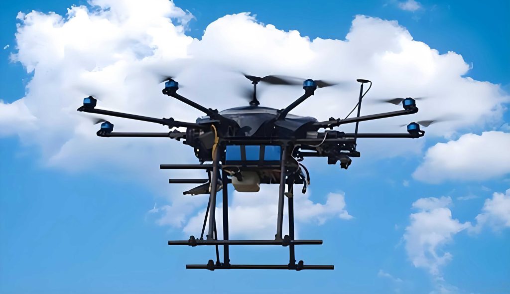
However, deploying UAV drones for systematic inspection in such environments is not trivial. A critical challenge lies in determining *where* to inspect. Blindly covering the entire area is inefficient and energy-prohibitive. Therefore, a risk-informed approach is essential to prioritize inspection efforts. Furthermore, planning an optimal flight path for the UAV drones in three-dimensional space, considering their physical constraints and energy consumption, is a complex optimization problem. The goal is to generate a flight route that visits all high-priority locations while minimizing total energy expenditure, thereby maximizing the operational endurance and coverage of a single flight.
This work presents an integrated framework that combines multi-factor risk assessment with advanced 3D path planning for UAV drones tasked with scenic area safety inspection. Our strategy involves first identifying and quantifying risk across the area to define critical inspection points, and then solving for the most energy-efficient flight path connecting these points, adhering to the realistic flight dynamics of UAV drones.
1. Risk-Informed Inspection Node Selection
The first pillar of our framework is the objective identification of high-risk zones within the scenic area, which subsequently serve as the mandatory nodes (target points) for the UAV drones’ inspection path. We move beyond single-hazard assessments to a holistic, multi-dimensional risk evaluation.
1.1. Grid-Based Environmental Modeling and Risk Factor Identification
To systematically analyze the heterogeneous landscape, the scenic area is discretized using a grid-based method. The entire region is overlaid with a mesh of uniform square cells. The size of each grid cell is determined by balancing the need for spatial detail with practical considerations such as the camera’s field of view of the UAV drones and the typical scale of points of interest.
We identify a comprehensive set of risk factors (Ca) that contribute to the likelihood or severity of safety incidents, categorized into three primary groups:
| Primary Factor | Secondary Factor (Ca) | Description |
|---|---|---|
| Topography (C1) | Elevation (C11) | Lower altitudes often correlate with higher visitor density and complex traffic, increasing accident probability. |
| Crowd Aggregation (C2) | Visitor Flow (C21) | Higher foot traffic in popular spots elevates the risk of incidents like stampedes or conflicts. |
| Land Use Type (C22) | Different zones (e.g., facilities, forests, water bodies) have varying inherent risks and activity patterns. | |
| Rescue Conditions (C3) | Accessibility of Safety Channels (C31) | The presence and condition of roads/paths critical for emergency vehicle and personnel access. |
| Emergency Response Distance (C32) | Distance from the potential incident location to the nearest emergency service center. |
Each grid cell is then scored for every risk factor (Ca) based on predefined criteria (e.g., elevation bands, visitor flow thresholds). Higher scores indicate higher risk levels for that specific factor within that cell.
1.2. Objective Weight Assignment and Composite Risk Calculation
Not all risk factors contribute equally to the overall safety hazard. To avoid subjective bias in assigning importance, we employ the Entropy Weight Method. This is an objective weighting technique where the weight (wa) for each factor is derived from the information content (disparity) of its scores across all grid cells. A factor with scores that vary greatly across the area provides more information and thus receives a higher weight. The process is as follows:
First, a normalized decision matrix is constructed from the scores of all factors across all grids. The entropy value ea for the a-th factor is calculated:
$$ e_a = -\frac{1}{\ln(m)} \sum_{j=1}^{m} p_{aj} \ln(p_{aj}) $$
where m is the number of grid cells, and paj is the proportion of the score of factor a in cell j relative to the sum of its scores across all cells.
The degree of divergence da for the factor is:
$$ d_a = 1 – e_a $$
Finally, the objective weight wa is obtained by normalizing the divergence:
$$ w_a = \frac{d_a}{\sum_{i=1}^{n} d_i} $$
where n is the number of risk factors (5 in our case).
The composite risk value R for each grid cell j is then computed as the weighted sum:
$$ R_j = \sum_{a=1}^{n} w_a \cdot C_{aj} $$
This calculation yields a quantitative risk map of the entire scenic area. Cells are ranked based on their composite risk value (Rj). The top-ranking cells (e.g., the highest 10%) are selected as the high-priority inspection nodes for the UAV drones. The central coordinates (x, y) and the terrain elevation (z) of these selected grids define the set of target points N for the path planning phase.
2. Energy-Minimizing 3D Path Planning Model for UAV Drones
With the set of inspection nodes N defined, the next challenge is to plan a flight path for the UAV drones that visits all nodes and returns to the start point, minimizing total energy consumption while respecting the aircraft’s physical limits.
2.1. UAV Drones Energy Consumption Modeling
A simplified force analysis model for a multi-rotor UAV drone is adopted, focusing on three primary flight modes: level flight, ascending flight, and descending flight. The primary forces considered are lift (F) and drag (Q). Based on empirical data from rotor tests, a relationship between the mechanical power output (P) and the generated lift (F) for UAV drones can be established. A fitted model is often expressed as:
$$ F = \alpha \cdot P^{\beta} + \gamma $$
where α, β, γ are coefficients derived from experimental data.
The energy efficiency coefficient E, defined as energy consumed per unit distance (J/m), is a crucial metric. It is derived from power and velocity (v):
$$ E = \frac{P}{v} $$
Therefore, distinct efficiency coefficients exist for different flight modes due to varying power requirements:
- Ef: Energy efficiency coefficient for level flight.
- Er: Energy efficiency coefficient for ascending flight (requires extra power to overcome gravity).
- Ed: Energy efficiency coefficient for controlled descending flight (may require less power than hovering).
The values for these coefficients are determined by substituting the lift force required to maintain the specific flight mode (which balances gravity and drag components) into the power-lift relationship and then applying the efficiency formula. The results for a typical small inspection UAV drone might be:
| Flight Mode | Lift Force F (N) | Power P (W) | Velocity v (m/s) | Efficiency Coefficient E (J/m) |
|---|---|---|---|---|
| Level Flight | ~2.45 | ~28.58 | 10.0 | Ef = 2.86 |
| Ascending Flight | ~2.56 | ~29.17 | 3.0 | Er = 9.72 |
| Descending Flight | ~2.32 | ~27.90 | 3.0 | Ed = 9.30 |
2.2. Optimization Model Formulation
The path planning problem is formulated as an Energy-Minimizing Traveling Salesman Problem (EM-TSP) in 3D space. The objective is to find a Hamiltonian cycle (a tour that visits each node in N exactly once and returns to the start) that minimizes total energy consumption.
Objective Function:
$$ \min T_d = \sum_{i=0}^{n-1} d(V_i, V_{i+1}) + d(V_n, V_0) $$
where Td is the total energy consumption (J), Vi ∈ N ∪ {V0} are the ordered nodes in the path (with V0 as the start/end depot), n = |N|, and d(Vi, Vi+1) is the energy cost to travel from node i to node i+1.
The segment energy cost d(Vi, Vi+1) is calculated based on the 3D displacement and the corresponding efficiency coefficient:
$$ d(V_i, V_{i+1}) = \frac{\sqrt{(x_{i+1}-x_i)^2 + (y_{i+1}-y_i)^2}}{E_f} + \begin{cases}
\frac{z_{i+1}-z_i}{E_r}, & \text{if } z_{i+1} \ge z_i \\
\frac{z_i – z_{i+1}}{E_d}, & \text{if } z_{i+1} < z_i
\end{cases} $$
where (xi, yi, zi) are the 3D coordinates of node Vi.
Operational Constraints:
- Maximum Range Constraint: The total physical flight distance L must be less than the UAV drone’s maximum endurance Lmax.
$$ L = \sum_{k=1}^{n+1} l_k \leq L_{max} $$ - Minimum Step Length Constraint: UAV drones require a minimum straight-line segment length lmin to stabilize after a change in heading.
$$ l_k \geq l_{min} $$ - Maximum Turning Angle Constraint: For stability and safe maneuvering, the turning angle φ at any node must not exceed a maximum allowable angle φmax. The angle is computed from consecutive path segments projected onto the horizontal plane.
$$ \phi_i = \arccos\left( \frac{\vec{P}_{i-1,i} \cdot \vec{P}_{i,i+1}}{|\vec{P}_{i-1,i}| \times |\vec{P}_{i,i+1}|} \right) \leq \phi_{max} $$
where $\vec{P}_{i-1,i}$ is the vector from node Vi-1 to Vi.
If a node in the initial solution violates the maximum turning angle constraint, the path is locally optimized by inserting a short auxiliary waypoint. This new point is placed at a distance lmin from the problematic node, at the maximum allowable angle φmax, ensuring both the angle constraint and the minimum step length are satisfied for the new segments.
3. Algorithmic Solution: The LKH Algorithm for UAV Drones Path Planning
Solving the EM-TSP, an NP-hard problem, for a practical number of inspection nodes requires an efficient and effective heuristic. We employ the Lin-Kernighan-Helsgaun (LKH) algorithm, renowned for its exceptional performance in solving large-scale TSP instances.
The LKH algorithm enhances the classical Lin-Kernighan local search procedure with sophisticated mechanisms tailored for UAV drones path planning:
- Candidate Set Generation: Instead of considering all possible edges between nodes, it uses the α-measure based on minimum 1-trees to create a restricted candidate set of promising edges, drastically reducing the search space.
- Iterative k-opt Moves: The core local search engine performs complex k-opt exchanges (removing and adding k edges) to escape local optima, dynamically increasing k to find deeper improvements.
- Effective Search Guidance: It utilizes sensitivity analysis information to guide the search and perturbs the current best tour to explore different regions of the solution space.
The workflow integrated into our UAV drones path planner is:
- Input & Preprocessing: Input the 3D coordinates of the depot and all high-risk inspection nodes. Generate the asymmetric cost matrix d(i,j) using the energy consumption formula.
- Initialization: The LKH algorithm generates an initial tour, often using a fast constructive heuristic like the minimum spanning tree-based method.
- Local Optimization: The algorithm iteratively applies LK moves to the current tour. It explores the candidate edge sets to find sequences of link exchanges that yield a lower total energy cost (Td).
- Path Validation & Correction: The resulting best tour is checked against the maximum turning angle constraint. Any violating node triggers the insertion of an auxiliary waypoint, and the affected path segments are re-evaluated.
- Output: The final, feasible 3D inspection path, the sequence of nodes, and the calculated total energy consumption are output.
4. Case Study: Application in a Mountainous Scenic Area
To validate the proposed framework, we applied it to a large, topographically complex national park. The area was divided into 247 grid cells of 150m x 150m. Data for the five risk factors were collected for each cell.
Applying the entropy weight method yielded the following objective weights, highlighting that visitor flow is the most influential risk factor in this context:
| Risk Factor (Ca) | Weight (wa) |
|---|---|
| Elevation (C11) | 0.0685 |
| Visitor Flow (C21) | 0.4095 |
| Land Use Type (C22) | 0.1253 |
| Safety Channel (C31) | 0.2655 |
| Response Distance (C32) | 0.1311 |
The composite risk map identified 25 highest-risk cells. These became the inspection nodes for the UAV drones. The flight parameters for a commercial multi-rotor UAV drone were set: vf=10 m/s, vr=vd=3 m/s, lmin=50 m, φmax=120°, Lmax=10 km. The energy efficiency coefficients were those calculated previously.
The LKH algorithm was executed to solve the EM-TSP. The initial solution required a path correction for one node where the turning angle exceeded 120°. After inserting an optimization waypoint, the final 3D inspection path for the UAV drones was obtained.
Results:
- Optimal Path Length: 8,620.66 meters.
- Minimum Energy Consumption (Td): 33,895.55 Joules.
- Computation Time: Approximately 2.35 seconds.
Performance Comparison: To benchmark the LKH algorithm’s efficacy for this UAV drones task, it was compared against three widely-used metaheuristics: Genetic Algorithm (GA), Ant Colony Optimization (ACO), and Grey Wolf Optimizer (GWO). Each algorithm was run 10 times on the same node set and cost matrix. The results clearly demonstrate the superiority of the LKH approach for this application.
| Algorithm | Avg. Runtime (s) | Best Energy Found (J) | Avg. Energy (J) | Std. Dev. (J) |
|---|---|---|---|---|
| LKH | 2.35 | 33,895.55 | 33,912.67 | 22.51 |
| Genetic Algorithm (GA) | 60.00 | 34,035.63 | 34,108.93 | 152.39 |
| Ant Colony Opt. (ACO) | 72.00 | 35,028.52 | 35,545.48 | 397.42 |
| Grey Wolf Opt. (GWO) | 4.77 | 38,437.53 | 39,605.64 | 3,159.23 |
The LKH algorithm not only found the lowest-energy path but also did so orders of magnitude faster than GA and ACO. Its minimal standard deviation across runs indicates exceptional solution stability and reliability—a critical feature for operational planning of UAV drones missions. While GWO was relatively fast, it converged to significantly poorer solutions with high variance.
5. Conclusion
This work has presented a robust, two-stage framework for intelligent safety inspection in scenic areas using UAV drones. The integration of a multi-factor, entropy-weighted risk assessment provides a data-driven, objective methodology for identifying critical areas that demand aerial surveillance. This ensures that the limited flight time of UAV drones is focused on the zones where it is most needed for preventive safety management.
Subsequently, formulating the inspection task as an Energy-Minimizing TSP with realistic kinematic constraints (like maximum turning angle) allows for the generation of practical and efficient flight paths. The adoption of the LKH algorithm as the solver proves highly effective, consistently generating optimal or near-optimal inspection routes for UAV drones with remarkable computational speed and reliability compared to common metaheuristics.
The case study demonstrates the practical applicability of the entire framework. The resulting path enables UAV drones to complete a comprehensive inspection of all high-risk locations with minimized energy expenditure, directly translating to longer potential flight times or the ability to use smaller, more agile UAV drones. This synergy of risk-aware planning and high-performance path optimization significantly advances the operational capacity for automated, efficient, and intelligent safety monitoring of complex scenic environments using UAV drones.