The precise measurement of earthwork volumes at disposal sites is a fundamental prerequisite for effective land reclamation, directly impacting project costing, resource allocation, and environmental compliance. Traditional surveying methods, primarily reliant on total stations or Real-Time Kinematic (RTK) Global Navigation Satellite Systems (GNSS), involve personnel physically traversing often unstable and hazardous terrain to collect discrete topographic points. This process is not only time-consuming and labor-intensive but also poses significant safety risks, such as the threat of collapses or falls on loose, uneven slopes. The spatial resolution of the resulting topographic model is inherently limited by the density of manually surveyed points, creating a trade-off between survey effort and calculation accuracy. The advent of affordable, high-performance UAV drones equipped with advanced imaging sensors offers a paradigm shift. This study demonstrates the comprehensive application of consumer-grade UAV drone oblique photogrammetry for generating high-precision three-dimensional (3D) reality-based models of an abandoned soil site, subsequently enabling efficient and accurate automated earthwork volume calculation. This methodology effectively addresses the shortcomings of conventional techniques by enhancing safety, dramatically improving field efficiency, and providing a dense, continuous representation of the terrain surface for superior volumetric analysis.
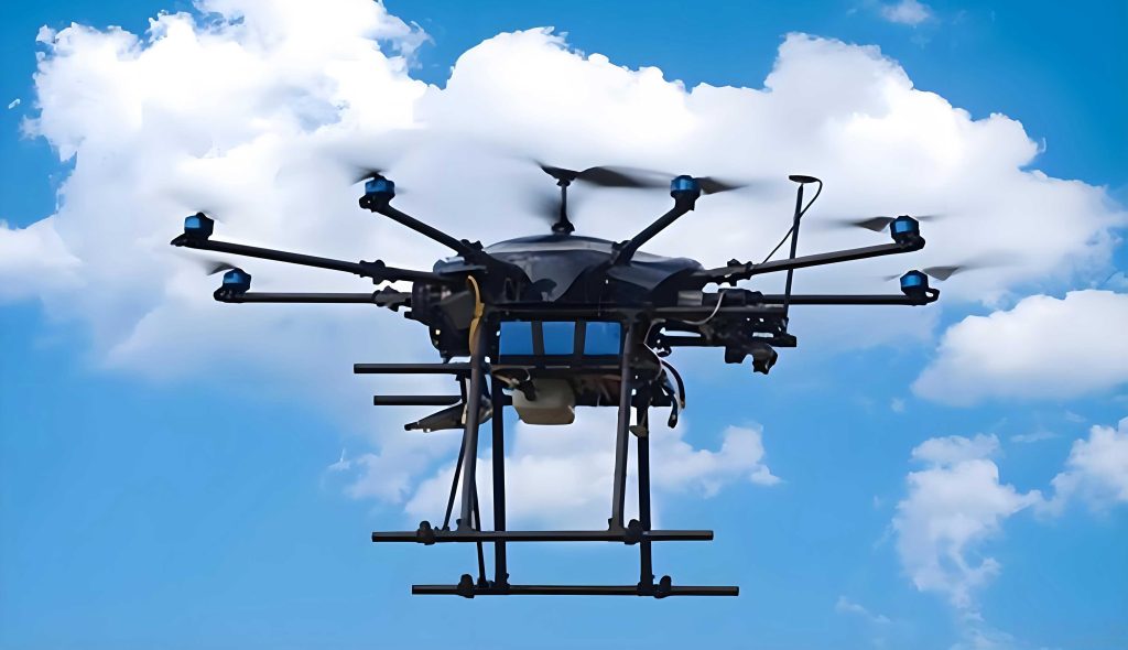
The selected study area is an abandoned soil site covering approximately 65,000 square meters, characterized by significant earth mounds, the tallest exceeding 4.5 meters in height. The variable and potentially unstable ground conditions made it an ideal candidate to demonstrate the safety and efficiency advantages of UAV drone technology over ground-based surveys. For this project, a DJI Phantom 4 RTK UAV drone was deployed. This platform integrates a centimeter-level positioning RTK module, which embeds highly accurate geospatial coordinates directly into each image’s metadata. This feature is crucial as it can obviate the need for extensive ground control point (GCP) networks, streamlining field operations considerably. Although equipped with a single-sensor camera, its gimbal allows for pitch control between -90° and +30°, enabling the simulation of a multi-view imaging system essential for oblique photogrammetry.
The mission was meticulously planned to ensure complete coverage and high model quality. A “lawnmower” (zigzag) flight pattern was employed with the camera nadir angle fixed at -45° to capture oblique imagery. The flight parameters were set to achieve a high overlap: 80% frontal overlap and 70% side overlap. Flying at a relative altitude of 75 meters resulted in a Ground Sampling Distance (GSD) of approximately 1.91 cm, sufficient for 1:500 scale mapping accuracy. The entire aerial survey, capturing 454 multi-view images, was completed in under 40 minutes of total field time, a task that would have required multiple days using traditional methods while exposing personnel to site hazards.
The core of photogrammetric processing lies in solving the collinearity equations to reconstruct the 3D scene. For a point \(P(X, Y, Z)\) in object space and its corresponding image point \(p(x, y)\), the relationship is given by:
$$
\begin{aligned}
x – x_0 &= -f \frac{m_{11}(X – X_0) + m_{12}(Y – Y_0) + m_{13}(Z – Z_0)}{m_{31}(X – X_0) + m_{32}(Y – Y_0) + m_{33}(Z – Z_0)} \\[6pt]
y – y_0 &= -f \frac{m_{21}(X – X_0) + m_{22}(Y – Y_0) + m_{23}(Z – Z_0)}{m_{31}(X – X_0) + m_{32}(Y – Y_0) + m_{33}(Z – Z_0)}
\end{aligned}
$$
where \((X_0, Y_0, Z_0)\) are the coordinates of the perspective center, \(f\) is the focal length, \((x_0, y_0)\) are the coordinates of the principal point, and \(m_{ij}\) are the elements of a 3D rotation matrix derived from the angular orientation \((\omega, \phi, \kappa)\) of the image. The embedded RTK coordinates from the UAV drone provided strong initial values for \((X_0, Y_0, Z_0)\), enhancing the bundle adjustment solution.
The collected imagery was processed using Pix4D Mapper software with the “3D Maps” template. The software automatically performs aerial triangulation, dense image matching, and 3D reconstruction. The key outputs were a dense point cloud (over 50 million points), a Digital Surface Model (DSM), a Digital Orthophoto (DOM), and a textured 3D mesh model. The quality report indicated excellent geolocation accuracy, with over 99% of reprojection errors in X and Y under ±0.01 m and 94% in Z under ±0.03 m, validating the precision of the UAV drone RTK data.
The geometric fidelity of the generated 3D model was quantitatively assessed by comparing dimensions of identifiable features measured in the model against direct field measurements. Ten vertical and ten horizontal features (e.g., building dimensions, road markings) were used. The root mean square error (RMSE) for vertical distances was 0.16 m, and for horizontal distances was 0.10 m. The vertical accuracy conforms to Grade I standards for 1:500 scale 3D geographic models. The results are summarized in the table below.
| Feature Type | Number of Samples | RMSE (m) | Compliance with 1:500 Grade I Standard (<0.25m) |
|---|---|---|---|
| Vertical Distances | 10 | 0.16 | Yes |
| Horizontal Distances | 10 | 0.10 | N/A (No explicit standard) |
For earthwork calculation, the dense point cloud was exported and processed in LiDAR360 software, chosen for its robustness in handling massive point datasets. The workflow involved two critical steps: 1) Defining the Measurement Boundary: A precise polygon was digitized to clip the point cloud, excluding peripheral features like tall trees that would distort volume calculations. 2) Establishing the Reference Plane: The project requirement was to level the site to the grade of an existing adjacent road. Consequently, a reference plane was defined by manually selecting three non-collinear points on the road surface within the point cloud. The equation of this plane, \(Ax + By + Cz + D = 0\), served as the datum for cut and fill calculations. The perpendicular distance \(d\) from any point \(P(x_p, y_p, z_p)\) to this plane is:
$$
d = \frac{|Ax_p + By_p + Cz_p + D|}{\sqrt{A^2 + B^2 + C^2}}
$$
This distance represents the cut (if positive) or fill (if negative) height at that point relative to the design plane.
LiDAR360 employs a grid-based method for volume computation. The bounded area is subdivided into a regular grid of cells. The volume for each cell is calculated based on the difference between the average elevation of points within that cell and the elevation of the reference plane at the cell’s location. The total volume \(V\) is the sum of all cell volumes:
$$
V = \sum_{i=1}^{n} ( \bar{z}_{cell_i} – z_{plane_i} ) \cdot A_{cell}
$$
where \(A_{cell}\) is the area of a grid cell, \(\bar{z}_{cell_i}\) is the average elevation of points in cell \(i\), and \(z_{plane_i}\) is the elevation of the reference plane at the center of cell \(i\). The choice of grid cell size (\(A_{cell}\)) critically influences both computational efficiency and result accuracy.
To analyze this trade-off, volume calculations were performed using grid sizes ranging from 0.05 m to 0.35 m. The results, using the 0.05 m grid as the benchmark for highest accuracy, are presented in the following table.
| Grid Size (m) | Computation Time (s) | Cut Volume (m³) | Fill Volume (m³) | Cut Error vs. 0.05m (%) | Fill Error vs. 0.05m (%) |
|---|---|---|---|---|---|
| 0.05 | 278 | 81,614.8 | 49,489.7 | 0.0 | 0.0 |
| 0.10 | 95 | 82,468.8 | 49,951.2 | +1.0 | +0.9 |
| 0.15 | 56 | 83,236.2 | 50,474.3 | +2.0 | +2.0 |
| 0.20 | 41 | 83,800.9 | 51,102.4 | +2.6 | +3.2 |
| 0.25 | 29 | 84,598.6 | 51,530.9 | +3.6 | +4.0 |
| 0.30 | 25 | 85,461.4 | 51,960.9 | +4.5 | +4.8 |
| 0.35 | 23 | 85,773.1 | 52,729.0 | +4.9 | +6.2 |
The analysis reveals a clear pattern: increasing the grid size reduces computation time but leads to an overestimation of both cut and fill volumes. This overestimation occurs because larger grids generalize local terrain variations, smoothing out depressions and peaks. For high-precision applications where error must be kept below 1%, a grid size of 0.10 m is recommended. For general engineering purposes accepting errors of 3-5%, grid sizes between 0.15 m and 0.30 m offer an optimal balance, achieving computation times under a minute with acceptable accuracy. The 0.35 m grid, with a fill error exceeding 6%, demonstrates the risk of excessive generalization leading to potentially significant costing errors.
The integration of UAV drone technology with modern photogrammetric and point cloud processing software delivers transformative benefits for earthwork measurement in land reclamation and civil engineering projects. The primary advantages are multi-faceted:
- Enhanced Safety & Field Efficiency: UAV drones eliminate the need for personnel to access dangerous terrain, mitigating risks of injury. The field data acquisition for a 65,000 m² site was completed in roughly 40 minutes, a task orders of magnitude faster than traditional topographic surveys.
- Superior Data Density and Model Accuracy: Unlike sparse discrete points, photogrammetry generates a continuous, high-resolution 3D surface model comprising millions of data points. This captures terrain intricacies with far greater fidelity, forming a more reliable basis for volumetric calculations.
- High Automation and Workflow Integration: The processing pipeline, from UAV drone image capture to 3D model and final volume report, is highly automated. Software solutions like Pix4D Mapper and LiDAR360 feature streamlined workflows that minimize manual intervention, reduce processing time, and limit potential for human error.
- Informed Decision-Making through Parametric Analysis: The digital nature of the results allows for easy “what-if” scenario testing. The impact of key calculation parameters, such as grid size, can be quantitatively assessed to align the workflow with specific project accuracy and efficiency requirements.
The following table synthesizes a comparative analysis of key project metrics, highlighting the transformative impact of the UAV drone-based methodology.
| Metric | Traditional GNSS/Total Station Method (Estimated) | UAV Drone Photogrammetry Method (This Study) | Improvement / Advantage |
|---|---|---|---|
| Field Data Acquisition Time | 2-3 Days | ~40 Minutes | ~95% Reduction |
| Personnel On-Site Risk | High (Unstable slopes) | Very Low (Remote operation) | Major Safety Enhancement |
| Data Point Density | Sparse (Hundreds to thousands of points) | Extremely Dense (~50 million points) | Superior Terrain Representation |
| Primary Output | 2D Contour Map / Sparse TIN | True 3D Textured Mesh & Dense Point Cloud | Richer Deliverable for Visualization & Analysis |
| Volumetric Calculation Basis | Interpolation between sparse points | Direct computation from continuous surface | Objectively Higher Accuracy Potential |
| Parameter Sensitivity Testing | Difficult and Time-Consuming | Rapid and Automated (e.g., Grid Size analysis) | Informed Optimization of Calculations |
In conclusion, this study conclusively demonstrates that consumer-grade UAV drones, when coupled with RTK positioning and robust processing software, constitute a mature, reliable, and superior solution for earthwork volume measurement at sites like abandoned soil fields. The methodology delivers unprecedented combinations of speed, safety, and precision. The ability to generate a photorealistic 3D record of the site also provides invaluable documentation for project management, stakeholder communication, and monitoring change over time. As UAV drone technology continues to evolve, becoming more accessible and capable, its role as an indispensable tool in the surveyor’s and engineer’s toolkit is firmly established, paving the way for more efficient, safe, and data-driven construction and land management practices.