The increasing density of urban infrastructure and population has elevated the potential consequences of fires, making effective and proactive patrols a critical component of urban fire safety management. Traditional fire patrol methods, reliant on manual inspections or fixed camera surveillance, suffer from inefficiencies, limited coverage, and delayed response times. Fire-fighting Unmanned Aerial Vehicles (Fire UAVs) offer a promising alternative due to their high efficiency, low operational cost, and flexible mobility. Deploying a network of Fire UAVs for routine aerial surveillance can significantly enhance early fire detection and monitoring capabilities.
However, to fully realize the potential of Fire UAVs in urban fire patrol, a significant challenge must be addressed: the spatial heterogeneity of fire risk across different urban areas. A one-size-fits-all patrol strategy is inefficient. Regions with higher fire risk, such as those with dense populations, aged infrastructure, or concentrations of hazardous materials, necessitate more frequent and longer-duration surveillance compared to lower-risk zones. This variability directly influences core operational planning decisions, namely, where to base the Fire UAVs (facility location) and how to route them to cover all required areas (path planning). These two interrelated decisions form the classic Location-Routing Problem (LRP). Therefore, it is essential to develop an integrated optimization model that incorporates dynamic fire risk assessments to design a cost-effective and reliable Fire UAV patrol network. This study aims to construct a Fire UAV patrol location-path planning scheme that dynamically adjusts patrol frequency and dwell time based on quantified fire risk levels.
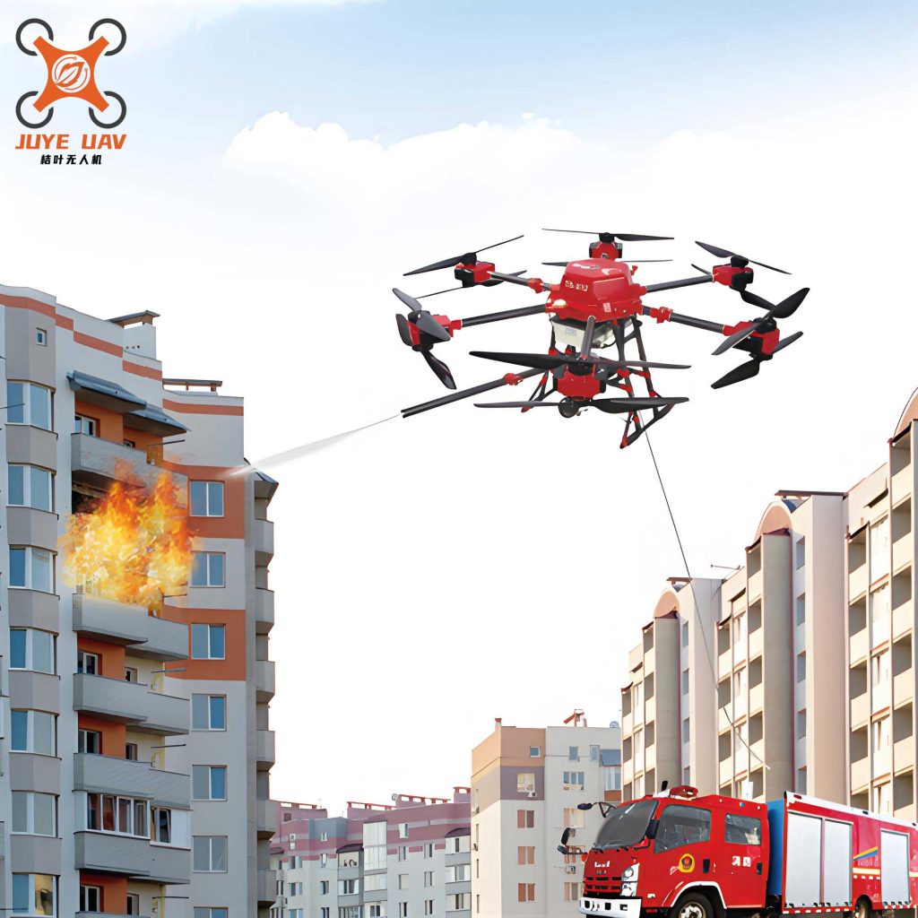
The envisioned Fire UAV patrol operation involves multiple UAVs launching from selected ground stations (e.g., existing or new fire stations). Each Fire UAV follows a pre-planned route, visiting multiple patrol demand points (representing specific geographic zones), spending a designated time conducting surveillance at each point, and finally returning to its origin station for recharging or maintenance. The entire network must satisfy the surveillance “demand” for every zone within a defined planning cycle. This operational scenario is depicted below.
1. Determination of Patrol Demand Points Based on Fire Risk Assessment
The foundation of the Fire UAV patrol planning model is a spatially explicit assessment of urban fire risk. This assessment translates qualitative hazard factors into quantitative demand inputs for the optimization model.
1.1 GIS-Based Urban Fire Risk Assessment
Geographic Information Systems (GIS) provide a powerful platform for integrating, analyzing, and visualizing spatial data related to fire hazards. The process involves compiling multi-source geospatial data, standardizing indicators, and applying a weighted overlay analysis to generate a composite fire risk map.
1.1.1 Fire Risk Evaluation Indicators: Based on established norms like the “Code for Urban Fire Protection Planning” (GB 51080-2015) and relevant literature, six key indicators were selected, categorized by ignition potential, vulnerability of assets, and rescue capability. These are summarized in Table 1.
| Indicator | Description & Rationale |
|---|---|
| Population Density | High density areas face greater risk of congestion and secondary incidents during evacuation. |
| Nighttime Light Intensity | Correlates with nighttime human activity and commercial density, indicating higher exposure risk during off-hours. |
| Fire Station Service Coverage | Areas within quick response distance have higher mitigation capacity; remote areas have higher potential for loss. |
| High-Risk Fire Buildings | Buildings with high fire load, complex structures, or occupancy that can lead to catastrophic casualties. |
| Building Height | Taller buildings pose greater challenges for firefighting and require longer evacuation times. |
| Building Age | Older buildings often have lower耐火等级, aged electrical wiring, and a higher probability of unpermitted modifications. |
1.1.2 Data Sources & Processing: Data for the six indicators were sourced from platforms including Gaode Map API (POIs and road networks), OpenStreetMap, national geographic databases, Earth Observation Group (night lights), national census data, and official fire department lists. Each indicator layer was processed within ArcGIS Pro, normalized, and classified into five risk grades using the Natural Breaks method.
1.1.3 Layer Overlay & Risk Mapping: Assuming equal importance for initial assessment, the five graded layers were combined using a weighted overlay tool in ArcGIS Pro. This synthesis produced a composite fire risk map with five distinct risk levels (1=Lowest to 5=Highest) for the study area.
1.2 Defining Patrol Demand Points
To transform the continuous risk map into discrete inputs for the Fire UAV routing model, the area corresponding to each risk level was tessellated into grids. The grid size is inversely related to the risk level, ensuring finer resolution for higher-risk zones: Level 5 (800m×800m), Level 4 (1000m×1000m), Level 3 (1200m×1200m), Level 2 (1400m×1400m), and Level 1 (1600m×1600m). The centroid of each grid cell is extracted as a patrol demand point $i \in I$, where $I$ is the set of all demand points. The risk level of the grid determines the patrol parameters for its centroid.
2. Fire Risk-Based Fire UAV Location-Routing Model
The core problem is formulated as a Mixed-Integer Quadratically Constrained Programming (MIQCP) model. The model simultaneously decides: (1) which candidate fire stations to activate as Fire UAV bases $s \in S$, (2) the set of patrol routes $r \in R$ originating from these bases, (3) the frequency $F_r$ at which each route is flown per planning cycle, and (4) the dwell time $T_{ir}$ a Fire UAV spends at each demand point $i$ on route $r$.
2.1 Assumptions and Notation
Key assumptions include: homogeneous Fire UAV fleet; negligible impact of minor weather variations on flight energy consumption; stable fire risk levels and patrol demand during the planning cycle; predefined flyable paths ignoring temporary no-fly zones; and patrol time considered as part of the flight phase as the Fire UAV moves within the grid. Main model sets, variables, and parameters are defined in Table 2.
| Type | Symbol | Description |
|---|---|---|
| Sets | $I$ | Set of patrol demand points. |
| $H \subset I$ | Subset of high-risk demand points. | |
| $S$ | Set of candidate Fire UAV base (station) locations. | |
| $R$ | Set of candidate patrol routes. | |
| Variables | $X_{ijr}$ | Binary, =1 if route $r$ travels from $i$ to $j$. |
| $A_r$ | Binary, =1 if route $r$ is activated. | |
| $B_s$ | Binary, =1 if base $s$ is activated. | |
| $P^{max}$ | Maximum patrol completion time among all routes. | |
| $T_{ir}$ | Dwell time (min) at point $i$ on route $r$. | |
| $F_r$ | Patrol frequency (sorties/cycle) for route $r$. | |
| $P^{in}_{ir}$ | Remaining battery (min) when Fire UAV arrives at $i$ on $r$. | |
| $P^{out}_{ir}$ | Remaining battery (min) when Fire UAV departs $i$ on $r$. | |
| $T_r$ | Total time (flight + dwell) for route $r$. | |
| $R^{ed}$ | Total patrol demand redundancy for high-risk points. | |
| Parameters | $C^r, C^s, C^c$ | Fixed cost for a route, a base, and a charging event. |
| $C^e$ | Energy cost per minute of flight. | |
| $\mu_i$ | Surveillance demand for point $i$ (time fraction). | |
| $l_i, u_i$ | Min and max single-visit dwell time at point $i$. | |
| $q$ | Fire UAV battery endurance (minutes). | |
| $t_{ij}$ | Flight time from point $i$ to $j$. | |
| $\omega$ | Cycle-to-week time conversion factor. | |
| $v, m$ | Fire UAV speed and mass. | |
| $\phi, \sigma$ | Propeller efficiency and lift-to-drag ratio. | |
| $\alpha, \beta, \gamma$ | Weight coefficients for multi-objective aggregation. |
2.2 Model Formulation
The model integrates three objectives: minimizing total system cost, minimizing the maximum patrol completion time to improve resource turnover, and maximizing safety coverage for high-risk areas by encouraging patrol time beyond the minimum demand.
Objective Function:
The aggregate objective function is:
$$ \min f = \alpha f_1 + \beta f_2 – \gamma f_3 $$
where:
$$ f_1 = \omega \left[ \sum_{r \in R} A_r C^r + \sum_{s \in S} B_s C^s + \sum_{r \in R} F_r (C^c + C^e T_r) \right] $$
$$ f_2 = P^{max} $$
$$ f_3 = R^{ed} = \sum_{h \in H} \left( \sum_{r \in R} T_{hr} F_r – \mu_h \right) $$
The term $C^e T_r$ calculates the energy cost per sortie for route $r$, where $T_r$ includes both travel and dwell time. The redundancy $R^{ed}$ sums the excess patrol time allocated to all high-risk points.
Key Constraints:
1. Fire UAV Endurance & Routing:
$$ P^{out}_{ir} = P^{in}_{ir} – T_{ir} \quad \forall i \in I, r \in R $$
$$ P^{in}_{jr} \leq P^{out}_{ir} – t_{ij} + q(1-X_{ijr}) \quad \forall i,j, r $$
$$ P^{out}_{sr} = q B_s \quad \forall s \in S, r \in R $$
$$ T_r \geq q – P^{out}_{sr} \quad \forall s \in S, r \in R $$
These constraints track battery usage, ensure the Fire UAV starts with full battery from an open base, and guarantee sufficient charge to return.
2. Patrol Demand Satisfaction:
$$ \sum_{r \in R} T_{ir} F_r \geq \mu_i \quad \forall i \in I $$
$$ l_i \sum_{j} X_{ijr} \leq T_{ir} \leq u_i \sum_{j} X_{ijr} \quad \forall i \in I, r \in R $$
The first constraint ensures the total surveillance time meets the demand. The second enforces dwell time bounds. Note the quadratic term $T_{ir} F_r$.
3. Logic and Completeness:
$$ \sum_{i \in S} \sum_{j \in I} X_{ijr} = A_r \quad \forall r \in R $$
$$ \sum_{i \in I} \sum_{j \in S} X_{ijr} = A_r \quad \forall r \in R $$
$$ \sum_{i} X_{isr} = \sum_{j} X_{sjr} \quad \forall s \in S, r \in R $$
$$ \sum_{j} X_{ijr} = \sum_{j} X_{jir} \quad \forall i \in I, r \in R $$
These ensure each activated route starts and ends at the same open base, and flow conservation at each node.
4. Linking and Bounds:
$$ A_r \leq M F_r, \quad B_s \geq X_{isr} \quad \forall i,s,r $$
$$ A_r T_r \leq P^{max} \leq q \quad \forall r \in R $$
$$ R^{ed} \geq 0 $$
These link variables and define the maximum cycle time.
3. Solution Algorithm: Adaptive Large Neighborhood Search (ALNS)
The problem is decomposed. A master problem (selecting bases and routes) is solved using an ALNS heuristic, while a sub-problem (optimizing $F_r$ and $T_{ir}$ for a fixed route) is solved exactly via a greedy procedure.
3.1 Sub-Problem Solver
For a given route $r$ with ordered points, the sub-problem allocates dwell times $T_{ir}$ and determines frequency $F_r$. The algorithm checks feasibility against battery $q$, then iteratively allocates the usable time $t^{use} = q – \sum t_{ij}$ to points, first satisfying minimum times $l_i$, then distributing remaining time proportionally to demands $\mu_i$ to maximize efficiency. It yields the optimal $F_r^{*}$ and $T_{ir}^{*}$ for that route configuration.
3.2 ALNS for the Master Problem
The ALNS framework iteratively destroys and repairs solutions.
1. Initial Solution: A greedy heuristic opens bases covering the most unserved points and constructs routes by sequentially adding the nearest feasible point until battery limits are reached.
2. Destroy Operators: Remove points or routes from the current solution. Types include: Random Removal, Worst-Cost Removal, Route Removal, Base Removal, and Geographic Cluster Removal.
3. Repair Operators: Re-insert removed points into the partial solution. Types include: Random Insertion, Greedy Insertion (minimizing cost increase), and Regret-2 Insertion.
4. Adaptive Mechanism & Acceptance: Operator selection probabilities are updated based on their past performance using a roulette-wheel scheme. A simulated annealing criterion decides whether to accept a new solution, allowing escapes from local optima. The sub-problem solver is called within every destroy/repair step to evaluate route feasibility and cost.
4. Case Study and Analysis
The central six districts of Tianjin, China, were used as a case study (area: 195 km²). A fire risk map was generated, leading to 141 patrol demand points. Candidate bases were set at 45 existing fire stations. Fire UAV parameters were based on a commercial model (e.g., DJI Mavic Pro specs): endurance $q$=46 min, speed $v$=30 km/h, mass $m$=2 kg. Cost and other parameters are listed in Table 3.
| Parameter | Value | Parameter | Value |
|---|---|---|---|
| $m$ | 2 kg | $\alpha, \beta, \gamma$ | 0.5, 0.3, 0.2 |
| $v$ | 30 km/h | Initial Temperature | 1000 |
| $q$ | 46 min | Cooling Rate | 0.999 |
| $C^r$ | 20,000 | $C^s$ | 50,000 |
| $C^c$ | 15 | $C^e$ | 1.8 |
| $\phi$ | 0.5 | $\sigma$ | 3 |
4.1 Algorithm Validation
On small-scale instances (3-15 demand points), the ALNS solution was compared to the optimal solution from the Gurobi solver. ALNS achieved near-optimal results (average gap 1.4%) with drastically shorter computation time (seconds vs. minutes), demonstrating its effectiveness.
Further comparison with standard heuristics like Genetic Algorithm (GA), Particle Swarm Optimization (PSO), and Ant Colony Optimization (ACO) showed that ALNS provided better solution quality (lowest cost) and higher robustness (lower variance over multiple runs), making it most suitable for this Fire UAV patrol problem.
4.2 Baseline Patrol Network Solution
Patrol demand $\mu_i$ and dwell bounds $[l_i, u_i]$ were set according to risk level (Level 5: $\mu=0.3, [10,14]$; Level 1: $\mu=0.1, [16,20]$). The ALNS algorithm converged stably after about 1100 iterations. The optimized Fire UAV patrol network required activating 24 out of 45 candidate bases and operating 63 patrol routes. The total weekly system cost was approximately 4.30 million units. A subset of the resulting routes for one district is shown in Table 4.
| Base | Route Sequence | Dwell Times (min) | Freq ($F_r$) | Route Time $T_r$ (min) |
|---|---|---|---|---|
| 1 | ⑥ → ⑤ → ② | ⑥(13.32), ⑤(13.32), ②(11.67) | 0.023 | 44.59 |
| 1 | ⑨ → ⑬ → ⑧ | ⑨(13.38), ⑬(13.38), ⑧(13.38) | 0.025 | 44.53 |
| 3 | ⑩ → ⑭ → ③ | ⑩(13.99), ⑭(13.99), ③(11.33) | 0.023 | 44.12 |
4.3 Sensitivity Analysis
1. Impact of Fire UAV Endurance ($q$): Increasing endurance from 46 to 85 minutes reduced the total cost by ~20%, the number of required bases by ~42%, and the number of routes by ~54%. Longer flight time allows each Fire UAV to cover more points per sortie, consolidating the network.
2. Impact of Patrol Demand ($\mu_i$): A 67% increase in demand (e.g., from 0.3 to 0.5 for highest risk) raised the total cost by ~65%. The number of bases and routes remained stable, but the average patrol frequency $F_r$ increased by ~124% to meet the higher time requirements.
3. Impact of Dwell Time Bounds ($[l_i, u_i]$): Increasing the required dwell time per visit significantly altered the network. Raising $l_i$ and $u_i$ by +4 minutes increased the number of bases by ~129%, routes by ~93%, and cost by ~33%, while the average frequency dropped by ~88%. Longer mandatory dwells reduce how many points a Fire UAV can visit per battery charge, forcing a more decentralized network with more bases and routes flying less frequently.
5. Conclusion
This study developed an integrated framework for planning an urban Fire UAV patrol network. By first conducting a GIS-based fire risk assessment to define spatially differentiated surveillance demands, and then formulating and solving a novel MIQCP location-routing model, we demonstrated a practical approach for fire departments. The model successfully coordinates Fire UAV base selection, route design, patrol frequency, and dwell time allocation. The ALNS algorithm proved effective in solving this complex problem. The case study of Tianjin and the sensitivity analyses provide actionable insights: investing in Fire UAVs with longer endurance can significantly reduce infrastructure needs and cost, while surging patrol demands or longer inspection requirements per point will necessitate a larger, more distributed network of Fire UAV bases. Future work could integrate dynamic constraints such as real-time airspace obstacles, more refined energy consumption models for urban terrain, and uncertainty in fire risk forecasts.