
In the evolving landscape of modern naval warfare, the proliferation of unmanned aerial vehicles (UAVs) poses significant threats to maritime security. As a researcher focused on directed energy systems, I have dedicated substantial effort to evaluating the efficacy of shipborne laser weapons in countering these agile targets. This article presents a comprehensive simulation-based analysis of a ten-kilowatt class laser weapon system designed for anti-UAV operations. The primary objective is to assess the combat effectiveness under varying atmospheric conditions, providing a theoretical foundation for deployment and optimization. Through detailed modeling and Monte Carlo simulations, I explore critical factors such as atmospheric transmission effects, beam quality degradation, aiming accuracy, and damage thresholds. The focus remains on the anti-UAV capability, a term I will emphasize throughout to highlight the strategic importance of neutralizing drone threats.
The advent of laser weapons offers a paradigm shift in defensive tactics, enabling precise, scalable engagement with minimal collateral damage. For anti-UAV missions, lasers provide a graded response—from soft-kill options like dazzle or sensor degradation to hard-kill destruction—tailored to mission requirements. My investigation centers on a typical UAV target, analogous to the MQ-8C Fire Scout, to simulate real-world scenarios. By integrating atmospheric models with weapon performance parameters, I quantify the optimal engagement ranges and success probabilities. This work underscores the potential of laser systems as a cornerstone in future anti-UAV defenses, especially in maritime environments where conditions dynamically influence system performance.
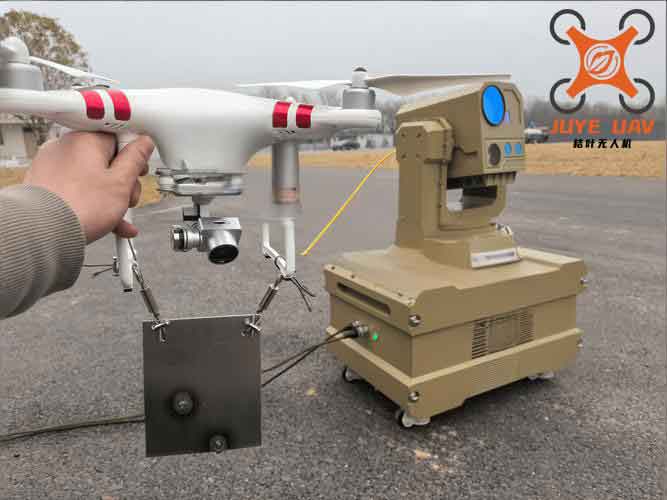
To contextualize this study, I first review the broader literature on laser weapon applications for anti-UAV roles. Prior research has extensively covered laser-material interaction mechanisms, atmospheric attenuation phenomena, and tracking system limitations. However, holistic simulations that combine these elements into a cohesive effectiveness model are less common. My approach builds on established physical principles but extends them through stochastic modeling to capture the uncertainties inherent in combat scenarios. The anti-UAV focus is critical, as drones often present small, fast-moving targets that challenge traditional kinetic systems. By leveraging high-fidelity simulations, I aim to bridge the gap between theoretical models and operational practicality.
The core of my methodology involves five interconnected modules: target equivalent modeling, atmospheric transmission modeling, on-target spot area modeling, on-target power and energy density modeling, and damage probability modeling. Each module incorporates key physics-based equations and empirical data to ensure realism. I employ a first-person perspective in describing these models, as if I were conducting the simulation myself. This narrative style enhances clarity and engagement, allowing readers to follow the logical flow from initial assumptions to final outcomes. Throughout, the term anti-UAV will recur to maintain thematic consistency and emphasize the application domain.
In the target equivalent model, I abstract the UAV as a point in a three-dimensional Cartesian coordinate system, simulating its motion as a straight-line trajectory with constant velocity. This simplification allows for tractable calculations while preserving essential dynamics. The target’s position is updated in real-time, enabling computation of the slant range and angles relative to the laser weapon. For instance, if the target has an initial position \((x_0, y_0, z_0)\) and a dive angle \(\theta_m\), its velocity components can be expressed as:
$$\frac{dx}{dt} = -V_m \cos \theta_m, \quad \frac{dy}{dt} = V_m \sin \theta_m, \quad \frac{dz}{dt} = 0$$
where \(V_m\) is the speed. The slant range \(R\) at any time is given by:
$$R = \sqrt{X^2 + Y^2 + Z^2}$$
after coordinate transformation to a geographic frame. This model supports both level and dive attacks, which are common in anti-UAV engagements.
The atmospheric transmission model accounts for two primary effects: attenuation due to absorption and scattering, and turbulence-induced beam degradation. For horizontal propagation, the transmittance \(T\) is often estimated using empirical relations tied to visibility \(V\). A widely used formula is:
$$T = \exp\left(-\frac{3.912 \times (0.55/\lambda)^q \times R}{V}\right)$$
where \(\lambda\) is the laser wavelength, and \(q\) is a correction factor dependent on visibility. For slant paths, a more complex expression incorporating zenith angle \(\theta\) is applied:
$$T = \exp\left(-\sec \theta \cdot K / V \cdot [1 – \exp(-0.835 R \cos \theta)]\right)$$
Here, \(K\) is an aerosol constant, typically 4.453 for maritime environments. Atmospheric turbulence, characterized by the refractive index structure constant \(C_n^2\), broadens the beam and reduces coherence. The coherence length \(r_0\) is calculated as:
$$r_0 = \frac{0.815 \lambda^{6/5}}{(C_n^2 R)^{3/5}}$$
leading to a beam quality factor \(\beta_t\):
$$\beta_t \approx \sqrt{1 + 0.62 (D / r_0)^{5/3}}$$
where \(D\) is the transmitter aperture. The combined beam quality \(\beta\) after accounting for initial quality \(\beta_f\) is:
$$\beta = \sqrt{\beta_f^2 + \beta_t^2}$$
These equations are pivotal for assessing how environmental conditions impact anti-UAV performance.
Next, the on-target spot area model determines the laser footprint on the UAV surface. The far-field spot radius \(r_1\) considers beam divergence and quality:
$$r_1 = \frac{1.22 \beta \lambda R}{D}$$
The projected area \(A\) depends on the engagement geometry—head-on or side attack. For head-on cases where the angle between beam and target is less than 30°, the area is:
$$A = \frac{\pi r_1^2}{|\cos \varepsilon \sin \beta|}$$
with \(\varepsilon\) and \(\beta\) as elevation and azimuth angles. For side attacks, a more general form applies. To incorporate aiming errors, I use Monte Carlo simulations, generating random deviations in elevation and azimuth that follow a normal distribution with zero mean and a standard deviation of 10 microradians. This stochastic approach yields the overlapping area \(S_J\) between the laser spot and target region, which is crucial for energy deposition calculations.
The on-target power and energy density models translate beam properties into potential damage. The attenuated power \(P_r\) at range \(R\) is:
$$P_r = P_0 T$$
where \(P_0\) is the emitted power. The power density \(I_r(t)\) on target is:
$$I_r(t) = \frac{K_1 P_r}{A}$$
with \(K_1 = 0.84\) as an energy concentration coefficient. The cumulative energy density \(E\) over an engagement duration from time 0 to \(n\) seconds is:
$$E = \frac{\sum I_r(t) S_J \sigma}{\pi r_2^2}$$
where \(\sigma = 0.8\) is the target material absorption coefficient, and \(r_2\) is the target radius (set to 0.01 m for critical components like sensors or fuel tanks). This energy metric, combined with power density, forms the basis of damage criteria.
Damage probability modeling defines success thresholds for anti-UAV engagements. I distinguish between soft-kill and hard-kill outcomes based on material vulnerabilities. For soft-kill, such as disabling electro-optical sensors, a lower power density threshold \(P_{r0}\) and longer exposure time are used. Hard-kill, involving structural failure, requires higher intensity. The criteria are:
$$\text{Success if: } I_r > P_{r0} \text{ and } E > E_0$$
where \(E_0 = P_{r0} \times T\) for a specified duration \(T\). To quantify effectiveness, I compute the probability of damage across the entire engagement envelope, iterating simulations to achieve statistical significance.
For simulation parameters, I assume a laser weapon with the following specifications, which are representative of current ten-kilowatt class systems:
| Parameter | Value |
|---|---|
| Wavelength (\(\lambda\)) | 1.06 \(\mu m\) |
| Initial Beam Quality (\(\beta_f\)) | 3 |
| Transmitter Diameter (\(D\)) | 0.3 m |
| Average Power (\(P_0\)) | 30 kW |
| Tracking Accuracy | 10 \(\mu rad\) |
The UAV target is modeled after typical reconnaissance drones, with key attributes summarized below:
| Attribute | Value |
|---|---|
| Max Speed | 260 km/h |
| Cruise Speed | 230 km/h |
| Max Altitude | 6100 m |
| Critical Component Size | 0.01 m radius |
Damage thresholds are derived from experimental data on common UAV materials, as shown in this table:
| Damage Type | Power Density Threshold (\(P_{r0}\)) | Energy Density Threshold (\(E_0\)) |
|---|---|---|
| Soft-Kill (e.g., sensor dazzle) | 70 W/cm² | 700 J/cm² (over 10 s) |
| Hard-Kill (e.g., structural burn-through) | 300 W/cm² | 1500 J/cm² (over 5 s) |
I conducted simulations for two atmospheric visibility conditions: 15 km and 25 km, representing moderate and good maritime environments. The UAV was set in a dive trajectory with initial conditions varied to test different engagement scenarios. Each simulation run involved 1000 Monte Carlo iterations to ensure robust probability estimates. The time step was 0.01 seconds, capturing dynamic interactions accurately.
The results reveal significant insights into anti-UAV performance. For soft-kill engagements, with the UAV starting at 3000 m altitude and 5000 m range in a 5° dive, the effective damage distance—where probability exceeds 99%—was 4380 m at 15 km visibility and 4890 m at 25 km visibility. The probability curves show a steep decline as range increases, underscoring the sensitivity to atmospheric attenuation. The mathematical relationship between visibility \(V\) and maximum damage range \(R_{\text{max}}\) can be approximated by fitting the data to an exponential decay model, highlighting how improved visibility extends reach.
For hard-kill scenarios, with initial parameters of 2000 m altitude and 2500 m range, the effective distances were 1720 m (15 km visibility) and 1990 m (25 km visibility). These shorter ranges reflect the higher energy requirements for structural damage. The probability curves exhibit similar trends but with lower baseline probabilities due to the stringent thresholds. To illustrate, I present a summarized table of results:
| Visibility (km) | Soft-Kill Range (m) | Hard-Kill Range (m) |
|---|---|---|
| 15 | 4380 | 1720 |
| 25 | 4890 | 1990 |
Furthermore, I explored the impact of increasing laser power to 100 kW, keeping other factors constant. This enhancement pushed the soft-kill range to approximately 7500 m and hard-kill to 3500 m under 25 km visibility, demonstrating that power scaling can partially mitigate atmospheric limitations. The relationship is nonlinear, as described by:
$$R_{\text{max}} \propto \ln(P_0) / \alpha(V)$$
where \(\alpha(V)\) is an attenuation coefficient dependent on visibility. This underscores the trade-offs in system design for anti-UAV missions.
Discussion of these findings emphasizes the critical role of environmental awareness in laser weapon deployment. For anti-UAV operations, commanders must factor in real-time visibility and turbulence data to optimize engagement decisions. My models show that even modest improvements in beam quality or tracking accuracy can yield disproportionate gains in success probability. Additionally, the graded damage approach allows for flexible responses—soft-kill might suffice for intelligence denial, while hard-kill is reserved for imminent threats. This adaptability makes lasers a versatile tool in the anti-UAV arsenal.
Limitations of this study include simplifications in target behavior (e.g., constant velocity, no evasive maneuvers) and atmospheric models (e.g., ignoring thermal blooming). Future work could incorporate more dynamic UAV trajectories and higher-fidelity weather simulations. Moreover, experimental validation with field tests would strengthen the model’s predictive power. Despite these constraints, the simulation framework provides a robust foundation for assessing laser weapon effectiveness in anti-UAV contexts.
In conclusion, my research demonstrates that ten-kilowatt shipborne laser weapons can be highly effective for anti-UAV missions, with engagement ranges varying significantly based on atmospheric conditions. Through integrated modeling of physics and stochastic processes, I quantified optimal interception radii and damage probabilities, offering actionable insights for naval planners. The anti-UAV capability is enhanced by the weapon’s scalability and precision, making it a promising component of layered defense systems. As drone threats evolve, continued refinement of such models will be essential to maintain tactical superiority. I advocate for further investment in laser technology and atmospheric research to fully realize its potential in safeguarding maritime domains.