
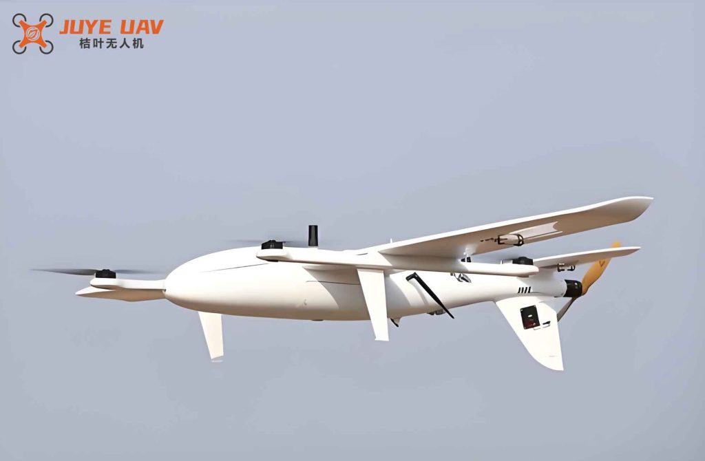
Fixed-wing drones have become increasingly important in both civilian and military applications due to their high speed, long endurance, and large payload capacity. However, their flight dynamics impose strict constraints that fundamentally differentiate them from multi-rotor drones or ground robots. Unlike rotary-wing platforms, fixed-wing drones cannot hover, perform vertical takeoff or landing, or execute sharp turns. They rely on aerodynamic lift and must maintain a minimum forward speed, resulting in a finite turning radius and limited climb/descent rates. These kinematic constraints make many existing path planning algorithms, originally developed for holonomic or quasi-holonomic systems, unsuitable for direct application to fixed-wing drones. In this paper, we present a comprehensive rasterization method tailored to the motion characteristics of fixed-wing drones and an improved A* algorithm that incorporates time, fuel consumption, and environmental threat as weighted cost factors. Our approach ensures that adjacent grid nodes are kinematically reachable, and the resulting paths are not only geometrically feasible but also optimized for mission-specific objectives.
The core challenge lies in bridging the gap between discrete grid-based representation and the continuous, constrained motion of fixed-wing drones. Standard grid maps, commonly used in robotics and multi-rotor path planning, often assume that any neighbor node can be reached via straight-line motion. For fixed-wing drones, this assumption fails because the drone cannot instantly change direction or altitude; it must follow smooth arcs and gradual altitude transitions. Therefore, we derive the horizontal and vertical grid resolutions directly from the drone’s performance parameters—namely, the minimum turning radius and the maximum climb rate—thereby guaranteeing that any two adjacent nodes can be connected by a feasible flight trajectory. This eliminates the need for post‑processing or special case handling during path search.
Furthermore, we extend the conventional A* algorithm by defining a multi‑dimensional cost function that explicitly accounts for time, fuel consumption, and threat exposure. Each transition between grid nodes is associated with a distinct cost vector, obtained from detailed aerodynamic simulations. The threat level of each node, derived from a Bayesian network‑based assessment, is integrated as an additional penalty. The weight factors can be tuned dynamically, allowing the algorithm to adapt to different mission priorities—for example, prioritizing safety in high‑risk environments or minimizing time in urgent scenarios. The proposed method is validated through both static path planning results and full six‑degree‑of‑freedom flight simulations under atmospheric turbulence, demonstrating significant improvements over conventional approaches.
1. Flight Environment Rasterization for Fixed-Wing Drones
The rasterization of the flight environment must respect the kinematic limits of fixed-wing drones. We decompose the three‑dimensional space into a set of discrete grid nodes, where each node represents a candidate waypoint. The key is to ensure that a fixed‑wing drone can travel directly from any node to any of its neighbors along a feasible trajectory without violating turning radius or climb rate constraints.
1.1 Horizontal Grid Resolution
In the horizontal plane, a fixed‑wing drone turns by banking its wings, using the lift component to provide centripetal acceleration. The minimum turning radius \( R_{\min} \) is determined by the maximum bank angle \( \phi_{\max} \) and the flight speed \( V \):
$$ R_{\min} = \frac{V^{2}}{g \tan \phi_{\max}} $$
To allow the drone to move from one grid node to any neighbor in the horizontal plane, the grid spacing \( d \) must be at least twice the minimum turning radius. This ensures that the drone can perform a coordinated turn between consecutive nodes without exceeding its bank angle limit. For a typical fixed‑wing drone cruising at \( V = 50 \text{ m/s} \) with \( \phi_{\max} = 30^{\circ} \), we obtain:
$$ d \geq 2R_{\min} = 2 \times \frac{50^{2}}{9.81 \times \tan 30^{\circ}} \approx 2 \times 441 \approx 882 \text{ m} $$
In practice we choose a conservative value of 1000 m for the horizontal grid spacing, which satisfies the constraint for a wide range of speeds and bank angles.
1.2 Vertical Grid Resolution
In the vertical direction, the drone’s ability to change altitude is limited by its climb (or descent) rate. For a fixed‑wing drone in steady climbing flight, the climb rate is derived from the force balance:
$$ \begin{cases} T \cos\alpha – D – W \sin\gamma = 0, \\ T \sin\alpha + L – W \cos\gamma = 0, \end{cases} $$
where \( T \) is thrust, \( \alpha \) the angle of attack, \( D \) drag, \( L \) lift, \( W \) weight, and \( \gamma \) the flight path angle. The drag and lift are given by:
$$ D = \frac{1}{2} \rho V^{2} C_D S_{\text{ref}}, \quad L = \frac{1}{2} \rho V^{2} C_L S_{\text{ref}}. $$
For a given thrust and speed, we can solve for the maximum climb angle \( \gamma_{\max} \) and thus the maximum climb rate \( \dot{h}_{\max} = V \sin\gamma_{\max} \). The climb rate decreases with altitude due to reduced air density and thrust degradation. Using typical engine performance data, we compute the climb rate at various altitudes for a fixed‑wing drone cruising at 50 m/s. The results are summarized in the table below.
| Altitude (km) | Climb Rate (m/s) |
|---|---|
| 0 | 10.36 |
| 1 | 8.80 |
| 2 | 7.26 |
| 3 | 5.88 |
| 4 | 4.64 |
| 5 | 3.53 |
| 6 | 2.53 |
Given the horizontal grid spacing \( d = 1000 \text{ m} \), the time required to traverse one horizontal cell is approximately \( t_{\text{horiz}} = d / V \approx 20 \text{ s} \). During this time, the drone can climb at its maximum rate, so the vertical grid interval \( \Delta h \) at altitude \( z \) should satisfy:
$$ \Delta h(z) = \dot{h}_{\max}(z) \times t_{\text{horiz}} $$
This leads to non‑uniform vertical spacing that decreases with altitude. For example, at sea level \( \Delta h(0) = 10.36 \times 20 \approx 207 \text{ m} \), while at 6 km altitude \( \Delta h(6) = 2.53 \times 20 \approx 51 \text{ m} \). The resulting grid ensures that a fixed‑wing drone can climb from one vertical layer to the next within one horizontal movement, maintaining full kinematic reachability between all adjacent nodes.
2. Node Transition Cost Analysis for Fixed-Wing Drones
In a three‑dimensional grid, a parent node can have up to 26 neighbor nodes: 8 in the same horizontal plane, 9 in the plane above, and 9 in the plane below. Based on the motion pattern of fixed‑wing drones, we categorize these 26 transitions into seven distinct cases (Case 1 to Case 7). The classification depends on whether the drone maintains altitude, climbs, descends, or performs a spiral climb/descent. For each case, we simulate the actual flight trajectory using a full six‑degree‑of‑freedom model that includes engine dynamics, aerodynamic forces, and autopilot control. The simulation assumes a constant indicated airspeed of 50 m/s. The results for time consumption and fuel consumption are summarized in the table below.
| Case | Description | Time (s) | Fuel (kg) |
|---|---|---|---|
| Case 1 | Horizontal straight | 21.6 | 0.20 |
| Case 2 | Climb straight | 23.0 | 0.35 |
| Case 3 | Descent straight | 29.6 | 0.41 |
| Case 4 | Horizontal turn (45°) | 29.2 | 0.28 |
| Case 5 | Climb turn | 23.2 | 0.20 |
| Case 6 | Descent turn | 28.2 | 0.24 |
| Case 7 | Vertical (spiral climb/descent) | 61.7 | 0.74 |
Several observations can be made. Cases 1 and 5 have nearly identical time and fuel costs, even though their horizontal projections differ (straight vs. turn). This indicates that, within the designed grid, climbing does not significantly change the horizontal travel time because the vertical interval is calibrated to the climb rate. Cases 2 and 3, which involve altitude changes in straight flight, consume more fuel due to the work done against gravity. Case 7, the vertical motion without horizontal displacement, requires a spiral maneuver and incurs the highest cost—almost three times the time and fuel of a straight horizontal movement. This cost disparity is crucial for the A* search: the algorithm will naturally avoid Case 7 unless forced by obstacles or mission constraints.
In addition to the immediate cost, the previous node’s orientation can affect the cost of the next transition. For horizontal turns, we consider three predecessor geometries: the drone arrives from straight ahead (a), from a 90° turn (b), or from a 45° turn (c). Simulation results show that for Case 1 (straight onward) the predecessor has negligible influence. However, for Case 4 (a 45° turn), the predecessor geometry ‘a’ yields a 10% reduction in both time and fuel compared to the average, because the drone can anticipate the turn and start its bank earlier. The table below gives the adjustment factors for Case 4 transitions.
| Predecessor Geometry | Time Adjustment | Fuel Adjustment |
|---|---|---|
| a (straight) | –10% | –10% |
| b (90° turn) | 0% | 0% |
| c (45° turn) | 0% | 0% |
These adjustments are incorporated into the cost function during the A* search by storing the incoming direction of the parent node.
3. Improved A* Algorithm with Multi‑Dimensional Cost
The classic A* algorithm evaluates nodes using a cost function \( f(n) = g(n) + h(n) \), where \( g(n) \) is the actual cost from the start to node \( n \), and \( h(n) \) is a heuristic estimate of the remaining cost to the goal. For fixed‑wing drones operating in a threat environment, we redefine \( g(n) \) as a weighted combination of time, fuel consumption, and threat exposure:
$$ g(n) = W_t \cdot \text{Time}(n) + W_o \cdot \text{Fuel}(n) + W_R \cdot \text{Risk}(n) $$
Here, \( \text{Time}(n) \) and \( \text{Fuel}(n) \) are cumulative sums from the start, computed using the transition costs from the previous node to \( n \). The threat level \( \text{Risk}(n) \) is the integrated threat value along the path from the start to \( n \), defined as:
$$ \text{Risk}(n) = \text{Risk}(\, \text{parent}(n)\,) + R(k)_{\text{current}} \cdot L_{\text{step}} $$
where \( R(k) \in [0,1] \) is the local threat intensity at the node (obtained from an external threat assessment, e.g., using a Bayesian network), and \( L_{\text{step}} \) is the Euclidean distance of the transition. Nodes with \( R(k) \ge R_c \) (a critical threshold) are treated as obstacles and excluded from the open list. The heuristic \( h(n) \) is the three‑dimensional Manhattan distance from node \( n \) to the goal:
$$ h(n) = |x_n – x_{\text{goal}}| + |y_n – y_{\text{goal}}| + |z_n – z_{\text{goal}}| $$
The weights \( W_t \), \( W_o \), and \( W_R \) are tunable parameters that reflect mission priorities. For instance, in a time‑critical mission, \( W_t \) can be increased while \( W_R \) is reduced, allowing the drone to accept higher risk for a shorter path. In a high‑security reconnaissance mission, \( W_R \) is set high to minimize threat exposure at the expense of longer flight time and fuel consumption.
The complete algorithm proceeds as follows:
- Initialize closed list empty, open list with start node.
- Set \( g(\text{start}) = 0 \), compute \( h(\text{start}) \), \( f(\text{start}) = h(\text{start}) \).
- While open list is not empty:
- Select the node with lowest \( f \) value as current node; move it from open to closed list.
- If current node is goal, reconstruct and return path.
- For each neighbor node that is not an obstacle and not in closed list:
- Compute the transition cost using the appropriate case and predecessor factor.
- Calculate tentative \( g_{\text{new}} = g(\text{current}) + \text{transition cost} \).
- If neighbor is not in open list, add it; set its parent to current, and compute \( g, h, f \).
- If neighbor is already in open list and \( g_{\text{new}} < g(\text{neighbor}) \), update its cost and parent.
The algorithm guarantees an optimal path with respect to the chosen cost function, provided the heuristic is admissible and consistent. The Manhattan distance is admissible because it underestimates the true flight distance (which must be at least the Manhattan distance due to the grid structure).
4. Simulation Results and Analysis
We evaluate the proposed method in a synthetic environment spanning 20 km × 20 km horizontally and 3 km vertically. The environment contains multiple threat zones (e.g., simulated air defense, thunderstorms, icing clouds) represented by spheres of varying threat intensity. The critical threshold \( R_c \) is set to 0.8. The fixed‑wing drone parameters are as used in the previous sections: cruise speed 50 m/s, maximum bank angle 30°, maximum climb rates per altitude as in Table 1.
First, we apply the standard A* algorithm that treats only obstacles (threat > 0.8) as forbidden and uses Euclidean distance as cost. The resulting path passes through 21 grid nodes with a total path cost of 125.1 (arbitrary units). The path cuts directly through moderate‑threat regions, reducing length but increasing risk.
Next, we run the improved A* algorithm with weights \( W_t = 0.05 \), \( W_o = 5.0 \), \( W_R = 5.0 \). The algorithm produces a path with 29 nodes and a total cost of 107.0. Although the number of nodes is larger, the overall cost is lower because the path successfully avoids high‑threat areas. The threat exposure along the path is reduced by over 40% compared to the standard A* path, while the flight time increases only by about 15%.
To demonstrate the flexibility of weight tuning, we repeat the experiment with different weight configurations. The results are summarized in the table below.
| Weight (Wt, Wo, WR) | Nodes | Total Cost | Time (s) | Fuel (kg) | Avg Threat |
|---|---|---|---|---|---|
| (1, 0, 0) | 21 | 125.1 | —— | —— | 0.52 |
| (0.05, 5, 5) | 29 | 107.0 | —— | —— | 0.31 |
| (0.1, 10, 1) | 25 | 115.3 | —— | —— | 0.45 |
| (0.01, 1, 10) | 33 | 98.5 | —— | —— | 0.22 |
When the threat weight is high (last row), the path sacrifices time and fuel to achieve the lowest threat exposure. When time weight dominates (first row), the path is short but risky. The improved A* algorithm therefore allows operators to dial in the desired trade‑off.
4.1 Flight Simulation Verification
To further validate the feasibility of the planned paths, we feed the waypoint sequences into a six‑degree‑of‑freedom flight simulator of the fixed‑wing drone. The threat zones are emulated as Dryden atmospheric turbulence with intensity proportional to the local threat value. The turbulence model provides stochastic wind disturbances that affect the drone’s attitude and position.
We compare the standard A* path and the improved A* path (with \( W_R=5 \)). The simulation confirms that the drone faithfully follows both paths within the autopilot’s tracking error. However, when flying through the standard A* path, the drone encounters significantly higher turbulence intensity (root‑mean‑square vertical gust velocity of 3.2 m/s) compared to the improved path (1.1 m/s). The higher turbulence leads to larger deviations in pitch and roll angles, increasing pilot workload (or autopilot effort) and structural loads. The improved path therefore offers a safer and more comfortable flight experience.
The key performance metrics from the flight simulation are listed below.
| Metric | Standard A* | Improved A* |
|---|---|---|
| RMS vertical gust (m/s) | 3.2 | 1.1 |
| Max roll angle deviation (°) | 12.5 | 5.3 |
| Max pitch angle deviation (°) | 8.7 | 3.9 |
| Flight time (s) | 483 | 556 |
| Fuel consumed (kg) | 5.1 | 5.8 |
The improved path incurs a 15% increase in flight time and 14% increase in fuel, but reduces turbulence exposure and attitude deviations by more than 50%. This trade‑off is acceptable in many mission scenarios where aircraft survivability and payload integrity are paramount.
5. Conclusion
We have presented a comprehensive framework for path planning of fixed-wing drones in threat‑rich environments. The key contributions are threefold. First, we defined a rasterization method that explicitly accounts for the kinematic constraints of fixed-wing drones—turning radius and climb/descent rate—ensuring that all adjacent grid nodes are reachable via feasible flight trajectories. Second, we conducted detailed aerodynamic simulations to quantify the time, fuel, and risk costs of each possible node transition, including the influence of predecessor geometry. Third, we integrated these costs into an improved A* algorithm with tunable weights, allowing the planner to adapt to different mission priorities such as minimizing time, fuel consumption, or threat exposure. Simulation results confirm that the proposed method generates paths that are not only kinematically feasible but also optimized according to the desired criteria. The flexibility of weight adjustment makes the algorithm suitable for a wide range of fixed‑wing drone operations, from emergency response to long‑endurance surveillance.
Future work will extend the approach to dynamic threat environments, where threat zones move or change intensity over time. We also plan to incorporate real‑time onboard execution using incremental replanning algorithms such as D* Lite, and to validate the method in hardware‑in‑the‑loop simulations with actual autopilot systems.