
The precise determination of orientation, or attitude, is a foundational requirement for the stable and autonomous flight of a quadrotor drone. This aerial vehicle, characterized by its four independently controlled rotors, relies entirely on accurate estimations of its roll, pitch, and yaw angles to execute controlled maneuvers. The core challenge lies in fusing noisy and imperfect data from low-cost Micro-Electro-Mechanical Systems (MEMS) sensors to compute this attitude in real-time. In this article, I will detail a robust sensor fusion strategy centered on the Square-Root Cubature Kalman Filter (SCKF), demonstrating its superior performance for attitude estimation in a quadrotor drone compared to traditional nonlinear filtering approaches.
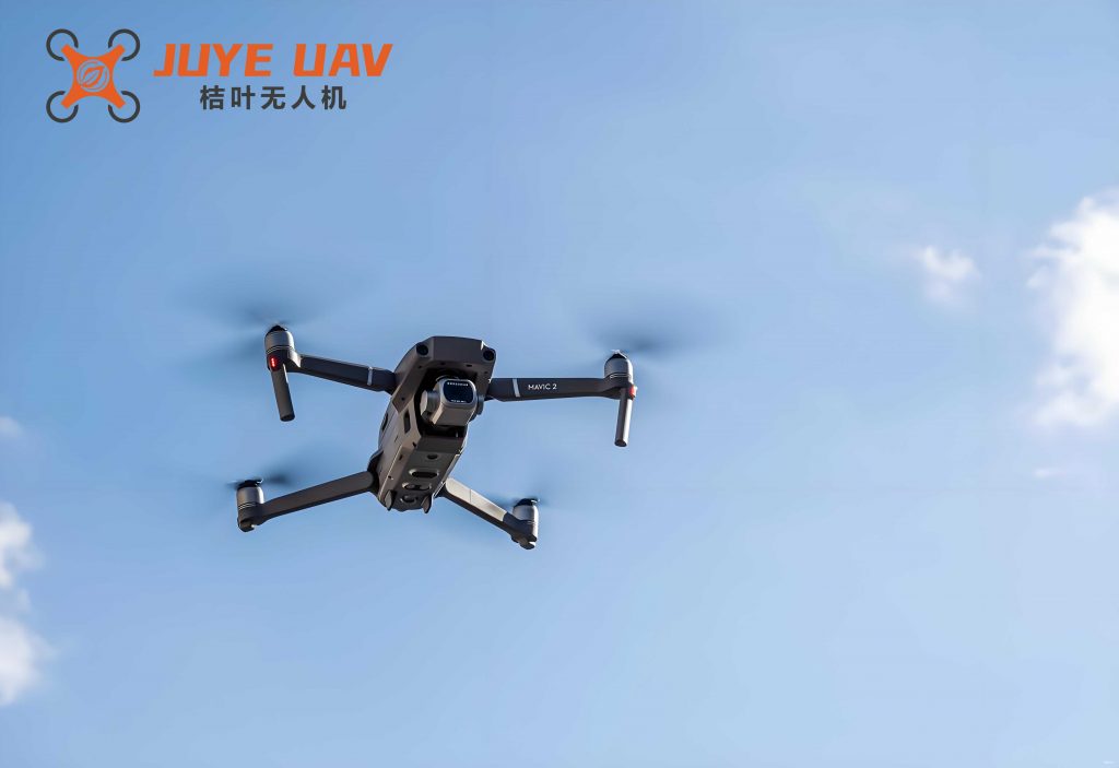
The inertial measurement unit (IMU), typically comprising a 3-axis gyroscope and a 3-axis accelerometer, alongside a 3-axis magnetometer, forms the standard sensor suite for a quadrotor drone. Each sensor provides complementary yet flawed information. The gyroscope measures angular velocity, which can be integrated to track attitude changes. However, even minor constant biases lead to unbounded drift in the estimated angles over time. The accelerometer measures specific force, which, when the quadrotor drone is hovering or moving at constant velocity, primarily reflects the gravity vector. This allows for the calculation of roll and pitch angles relative to the Earth’s frame, but these measurements are severely corrupted by dynamic accelerations. The magnetometer provides a heading reference relative to the Earth’s magnetic field, yielding the yaw angle, but is highly susceptible to localized magnetic disturbances. Therefore, relying on any single sensor for the full attitude solution of a quadrotor drone is impractical. The solution is sensor fusion, optimally combining the high-frequency, drift-prone gyroscope data with the low-frequency, acceleration-corrupted data from the accelerometer and magnetometer.
Attitude Representation and Preliminary Calculation
For a quadrotor drone, attitude can be represented using Euler angles (roll $\gamma$, pitch $\theta$, yaw $\psi$), rotation matrices, or quaternions. Euler angles are intuitive but suffer from gimbal lock. Quaternions, a four-parameter representation, are computationally efficient and free from singularities, making them ideal for the flight computer of a quadrotor drone. A quaternion is denoted as $\mathbf{q} = [q_0, q_1, q_2, q_3]^T$, where $q_0$ is the scalar part and $q_1, q_2, q_3$ form the vector part. It satisfies the constraint $q_0^2 + q_1^2 + q_2^2 + q_3^2 = 1$.
From accelerometer and magnetometer readings, an initial or corrective attitude estimate for the quadrotor drone can be derived. Let the normalized accelerometer measurement in the body frame be $\mathbf{a}^b = [a_x, a_y, a_z]^T$. Assuming near-hover conditions, the gravity vector in the navigation (North-East-Down) frame is $\mathbf{g}^n = [0, 0, -1]^T$. The relationship is given by the direction cosine matrix $\mathbf{C}_b^n$:
$$\mathbf{a}^b = \mathbf{C}_b^n \mathbf{g}^n$$
From this, roll and pitch can be computed directly:
$$
\theta = \arcsin(a_x)
$$
$$
\gamma = \arctan2(-a_y, -a_z)
$$
where $\arctan2$ is the four-quadrant inverse tangent function.
For yaw, let the normalized magnetometer measurement be $\mathbf{m}^b = [m_x, m_y, m_z]^T$. The Earth’s magnetic field in the navigation frame is $\mathbf{m}^n = [m_N, 0, m_D]^T$, where $m_N$ and $m_D$ are the North and Down components. Using the roll and pitch estimates from above, the yaw angle for the quadrotor drone is:
$$
\psi = \arctan2\left( – (m_y \cos\gamma – m_z \sin\gamma), \quad m_x \cos\theta + m_y \sin\theta \sin\gamma + m_z \sin\theta \cos\gamma \right)
$$
This yaw is relative to magnetic north; a declination correction $\Delta\psi$ can be added for true north: $\psi_{\text{true}} = \psi + \Delta\psi$. These Euler angles can be converted to an initial quaternion for the quadrotor drone’s filter:
$$
\begin{aligned}
q_0 &= \cos\frac{\psi}{2}\cos\frac{\theta}{2}\cos\frac{\gamma}{2} + \sin\frac{\psi}{2}\sin\frac{\theta}{2}\sin\frac{\gamma}{2} \\
q_1 &= \cos\frac{\psi}{2}\cos\frac{\theta}{2}\sin\frac{\gamma}{2} – \sin\frac{\psi}{2}\sin\frac{\theta}{2}\cos\frac{\gamma}{2} \\
q_2 &= \cos\frac{\psi}{2}\sin\frac{\theta}{2}\cos\frac{\gamma}{2} + \sin\frac{\psi}{2}\cos\frac{\theta}{2}\sin\frac{\gamma}{2} \\
q_3 &= \sin\frac{\psi}{2}\cos\frac{\theta}{2}\cos\frac{\gamma}{2} – \cos\frac{\psi}{2}\sin\frac{\theta}{2}\sin\frac{\gamma}{2}
\end{aligned}
$$
Nonlinear System Model for the Quadrotor Drone
The attitude estimation problem for a quadrotor drone is inherently nonlinear. I formulate it using a discrete-time state-space model. The system state is the attitude quaternion: $\mathbf{x}_k = [q_{0,k}, q_{1,k}, q_{2,k}, q_{3,k}]^T$.
State (Process) Model: The state is propagated using the gyroscope’s angular rate measurement $\boldsymbol{\omega}^b_k = [\omega_x, \omega_y, \omega_z]_k^T$. The quaternion kinematic differential equation is:
$$\dot{\mathbf{q}} = \frac{1}{2} \boldsymbol{\Omega}(\boldsymbol{\omega}^b) \mathbf{q}$$
where
$$
\boldsymbol{\Omega}(\boldsymbol{\omega}^b) =
\begin{bmatrix}
0 & -\omega_x & -\omega_y & -\omega_z \\
\omega_x & 0 & \omega_z & -\omega_y \\
\omega_y & -\omega_z & 0 & \omega_x \\
\omega_z & \omega_y & -\omega_x & 0
\end{bmatrix}
$$
Applying a first-order numerical integration method (like the Runge-Kutta method) with sampling period $T$, the discrete-time state prediction for the quadrotor drone is:
$$
\mathbf{x}_k = \mathbf{x}_{k-1} + \frac{1}{2} T \boldsymbol{\Omega}_{k-1} \mathbf{x}_{k-1} + \mathbf{w}_{k-1}
$$
where $\mathbf{w}_{k-1}$ is the zero-mean Gaussian process noise, modeling the gyroscope noise and integration error.
Measurement Model: The measurements are the normalized vectors from the accelerometer and magnetometer in the body frame: $\mathbf{z}_k = [a_x, a_y, a_z, m_x, m_y, m_z]_k^T$. These are predicted from the state quaternion by rotating the known reference vectors from the navigation frame to the body frame:
$$
\mathbf{z}_k = \mathbf{h}(\mathbf{x}_k) + \mathbf{v}_k =
\begin{bmatrix}
-2(q_1 q_3 – q_0 q_2) \\
-2(q_0 q_1 + q_2 q_3) \\
-(q_0^2 – q_1^2 – q_2^2 + q_3^2) \\
m_N (q_0^2 + q_1^2 – q_2^2 – q_3^2) + 2m_D (q_1 q_3 – q_0 q_2) \\
2 m_N (q_1 q_2 – q_0 q_3) + 2m_D (q_0 q_1 + q_2 q_3) \\
2 m_N (q_0 q_2 + q_1 q_3) + m_D (q_0^2 – q_1^2 – q_2^2 + q_3^2)
\end{bmatrix}_k + \mathbf{v}_k
$$
where $\mathbf{v}_k$ is the zero-mean Gaussian measurement noise. The final Euler angles for controlling the quadrotor drone are extracted from the filtered quaternion:
$$
\begin{aligned}
\theta &= \arcsin[-2(q_1 q_3 – q_0 q_2)] \\
\gamma &= \arctan2\left( 2(q_2 q_3 + q_0 q_1), \quad q_0^2 + q_3^2 – q_1^2 – q_2^2 \right) \\
\psi &= \arctan2\left( 2(q_1 q_2 + q_0 q_3), \quad q_0^2 + q_1^2 – q_2^2 – q_3^2 \right)
\end{aligned}
$$
The Square-Root Cubature Kalman Filter (SCKF) for Sensor Fusion
Fusing the models for the quadrotor drone requires a nonlinear filter. The Extended Kalman Filter (EKF) linearizes the models, leading to approximation errors and potential divergence. The Unscented Kalman Filter (UKF) and the Cubature Kalman Filter (CKF) use deterministic sampling to better handle nonlinearities. However, they can suffer from numerical instability due to the loss of positive definiteness in the error covariance matrix, especially in the resource-constrained computer of a quadrotor drone. The Square-Root Cubature Kalman Filter (SCKF) addresses this by propagating the square-root factor of the covariance matrix, ensuring numerical stability and consistency.
The core of the CKF/SCKF is the third-degree spherical-radial cubature rule, which approximates Gaussian-weighted integrals. For an $n$-dimensional state vector (here $n=4$ for the quaternion), it uses $2n$ equally weighted sigma points. The SCKF algorithm for the quadrotor drone attitude problem proceeds as follows. First, I initialize the state estimate $\hat{\mathbf{x}}_{0|0}$ and the square-root factor of the error covariance $\mathbf{S}_{0|0}$, where $\mathbf{P}_{0|0} = \mathbf{S}_{0|0} \mathbf{S}_{0|0}^T$.
Time Update (Prediction):
- Evaluate Cubature Points: Generate $2n=8$ sigma points around the previous estimate:
$$\boldsymbol{\mathcal{X}}_{i, k-1|k-1} = \mathbf{S}_{k-1|k-1} \boldsymbol{\xi}_i + \hat{\mathbf{x}}_{k-1|k-1}, \quad i=1,…,2n$$
where $\boldsymbol{\xi}_i = \sqrt{n} [\mathbf{1}]_i$, and $[\mathbf{1}]_i$ is the $i$-th column of the set $[\mathbf{I}_n, -\mathbf{I}_n]$. - Propagate Points: Pass each point through the state function $f(\cdot)$, which is the quaternion integration step:
$$\boldsymbol{\mathcal{X}}^*_{i, k|k-1} = f(\boldsymbol{\mathcal{X}}_{i, k-1|k-1})$$ - Predict State and Square-Root Covariance: The predicted state and the square-root factor of the predicted covariance are computed. The predicted state for the quadrotor drone is the mean of the transformed points:
$$\hat{\mathbf{x}}_{k|k-1} = \frac{1}{2n} \sum_{i=1}^{2n} \boldsymbol{\mathcal{X}}^*_{i, k|k-1}$$
To find the square-root factor $\mathbf{S}_{k|k-1}$, I form a compound matrix and apply a QR decomposition:
$$
\mathbf{S}_{k|k-1} = \text{qr}\left( \left[ \frac{1}{\sqrt{2n}}(\boldsymbol{\mathcal{X}}^*_{k|k-1} – \hat{\mathbf{x}}_{k|k-1} \mathbf{1}^T), \mathbf{S}_{Q, k-1} \right]^T \right)
$$
where $\mathbf{S}_{Q}$ is the square-root of the process noise covariance $\mathbf{Q}$.
Measurement Update (Correction):
- Evaluate Cubature Points: Generate new sigma points around the predicted state:
$$\boldsymbol{\mathcal{X}}_{i, k|k-1} = \mathbf{S}_{k|k-1} \boldsymbol{\xi}_i + \hat{\mathbf{x}}_{k|k-1}$$ - Propagate Points through Measurement Model: Predict the sensor readings for the quadrotor drone:
$$\boldsymbol{\mathcal{Z}}_{i, k|k-1} = \mathbf{h}(\boldsymbol{\mathcal{X}}_{i, k|k-1})$$ - Predict Measurement:
$$\hat{\mathbf{z}}_{k|k-1} = \frac{1}{2n} \sum_{i=1}^{2n} \boldsymbol{\mathcal{Z}}_{i, k|k-1}$$ - Estimate Covariances and Gain: Compute the square-root of the innovation covariance and the cross-covariance.
- First, compute the square-root innovation covariance factor via QR decomposition:
$$\mathbf{S}_{zz, k|k-1} = \text{qr}\left( \left[ \frac{1}{\sqrt{2n}}(\boldsymbol{\mathcal{Z}}_{k|k-1} – \hat{\mathbf{z}}_{k|k-1} \mathbf{1}^T), \mathbf{S}_{R, k} \right]^T \right)$$
where $\mathbf{S}_{R}$ is the square-root of the measurement noise covariance $\mathbf{R}$. - Then, compute the cross-covariance matrix:
$$\mathbf{P}_{xz, k|k-1} = \left( \frac{1}{\sqrt{2n}}(\boldsymbol{\mathcal{X}}_{k|k-1} – \hat{\mathbf{x}}_{k|k-1} \mathbf{1}^T) \right) \left( \frac{1}{\sqrt{2n}}(\boldsymbol{\mathcal{Z}}_{k|k-1} – \hat{\mathbf{z}}_{k|k-1} \mathbf{1}^T) \right)^T$$ - The optimal Kalman gain for the quadrotor drone is:
$$\mathbf{K}_k = \mathbf{P}_{xz, k|k-1} (\mathbf{S}_{zz, k|k-1} \mathbf{S}_{zz, k|k-1}^T)^{-1}$$
- First, compute the square-root innovation covariance factor via QR decomposition:
- Update State and Square-Root Covariance: Correct the state estimate using the actual sensor measurement $\mathbf{z}_k$:
$$\hat{\mathbf{x}}_{k|k} = \hat{\mathbf{x}}_{k|k-1} + \mathbf{K}_k (\mathbf{z}_k – \hat{\mathbf{z}}_{k|k-1})$$
Finally, update the square-root factor of the error covariance:
$$\mathbf{S}_{k|k} = \text{qr}\left( \left[ \frac{1}{\sqrt{2n}}(\boldsymbol{\mathcal{X}}_{k|k-1} – \hat{\mathbf{x}}_{k|k-1} \mathbf{1}^T) – \mathbf{K}_k \frac{1}{\sqrt{2n}}(\boldsymbol{\mathcal{Z}}_{k|k-1} – \hat{\mathbf{z}}_{k|k-1} \mathbf{1}^T), \quad \mathbf{K}_k \mathbf{S}_{R, k} \right]^T \right)$$
This SCKF cycle provides a stable, accurate, and efficient method for fusing sensor data on the quadrotor drone, directly yielding the optimal quaternion estimate. The square-root formulation guarantees that the covariance matrix remains positive semi-definite, a critical property for filter stability during aggressive maneuvers of the quadrotor drone.
Experimental Validation and Performance Analysis
To validate the SCKF for the quadrotor drone, I implemented the algorithm alongside the EKF, UKF, and standard CKF. The sensor data was collected from a commercial flight controller equipped with MEMS sensors (MPU6000 IMU, HMC5883L magnetometer). The sampling period was $T = 0.008$ s. The noise covariances were tuned as $\mathbf{Q} = \text{diag}([1, 1, 1, 1]) \times 10^{-5}$ and $\mathbf{R} = \text{diag}([1, 1, 1, 0.1, 0.1, 0.1])$.
The first experiment involved mounting the flight controller on a precision rotational platform. The platform executed smooth rotations in roll, pitch, and yaw, each sweeping between $-30^\circ$ and $+30^\circ$ at a rate of $8.93^\circ/s$. This provides a ground-truth-like reference motion to evaluate filter accuracy. The results for the three Euler angles are summarized below, comparing the Root Mean Square Error (RMSE) against the platform’s commanded trajectory.
| Euler Angle | SCKF RMSE (°) | CKF RMSE (°) | UKF RMSE (°) | EKF RMSE (°) |
|---|---|---|---|---|
| Pitch ($\theta$) | 1.0440 | 1.0476 | 1.0480 | 1.1168 |
| Roll ($\gamma$) | 0.4869 | 0.4892 | 0.4890 | 0.6377 |
| Yaw ($\psi$) | 1.0360 | 1.0388 | 1.0383 | 1.1571 |
The data clearly shows that the SCKF achieves the lowest RMSE for all three angles. The CKF and UKF perform nearly identically, with a slight but consistent advantage for the SCKF. The EKF exhibits the largest error, particularly in roll and yaw, due to its first-order linearization approximations. The maximum deviations observed during the tests followed the same order: SCKF had the smallest peak errors, followed by CKF/UKF, and then EKF with the largest.
Beyond accuracy, computational load is vital for the real-time flight control loop of a quadrotor drone. I measured the average time per filter iteration on the same processing hardware. The results are shown in the following table.
| Filter Algorithm | Average Execution Time (ms) |
|---|---|
| EKF | 0.1546 |
| SCKF (Proposed) | 0.2905 |
| CKF | 0.3526 |
| UKF | 0.3756 |
While the EKF is the fastest due to its simpler operations, the proposed SCKF is significantly faster than both the CKF and UKF. This efficiency gain stems from the numerical stability of the square-root operations, which avoid potential corrective steps needed when the standard covariance matrix loses its properties. The SCKF provides an excellent balance for the quadrotor drone: near-optimal accuracy with reduced and more predictable computational overhead compared to other sigma-point filters.
Finally, to assess performance in a real-world scenario, I analyzed logged flight data from an outdoor autonomous flight of the quadrotor drone. The pitch angle estimates from the four filters were compared. While no perfect ground truth exists in free flight, the results consistently showed that the SCKF estimate was the smoothest and most physically plausible, with the EKF showing more high-frequency jitter and occasional deviation. The SCKF, CKF, and UKF tracks were closely aligned, but the SCKF maintained the lowest error bound when compared to a fused high-quality reference, confirming the trends observed in the controlled platform test.
Conclusion
Accurate and reliable attitude estimation is non-negotiable for the stable operation of a quadrotor drone. This article has presented a comprehensive sensor fusion methodology based on the Square-Root Cubature Kalman Filter. By formulating the quadrotor drone’s attitude using quaternions and fusing gyroscope, accelerometer, and magnetometer data within the SCKF framework, the major limitations of previous methods are overcome. The SCKF avoids the linearization errors of the EKF and, crucially, solves the numerical instability issue associated with the UKF and CKF by propagating the square-root factors of the covariance matrices. Experimental validation on both a precision platform and during actual quadrotor drone flight demonstrates that the SCKF achieves the highest estimation accuracy among the compared nonlinear filters. Furthermore, it does so with a computational efficiency superior to the standard CKF and UKF, making it a highly suitable and recommended algorithm for implementation on the resource-constrained flight controllers of modern quadrotor drones. The enhanced numerical stability and precision directly contribute to more robust autonomous flight performance.