
The rapid evolution of military technology has placed unmanned aerial vehicles (UAVs), or military drones, at the forefront of modern defense strategy. These systems offer significant advantages in intelligence, surveillance, reconnaissance (ISR), and strike missions without risking pilot lives. However, the development of advanced military drone platforms is a complex and capital-intensive endeavor. Accurately predicting their development costs during the early conceptual and design phases is a critical challenge for program managers, budget analysts, and defense acquisition officials. Precise cost estimation is essential for effective resource allocation, program feasibility studies, and maintaining fiscal discipline within constrained defense budgets.
Traditional cost estimation methodologies, such as parametric cost models, often rely on linear or log-linear relationships derived from historical data. These models assume a predefined functional form, which may not capture the complex, nonlinear interactions between a military drone‘s design parameters and its ultimate development cost. While techniques like Artificial Neural Networks (ANNs) have been applied to model these nonlinearities, they possess inherent drawbacks. ANNs require large volumes of high-quality training data, their architecture selection lacks a rigorous theoretical foundation, and they are prone to overfitting, which compromises their generalization capability on new, unseen data. In the domain of military drone development, available historical cost data for completed programs is often limited, making data-hungry methods less reliable.
This article explores the application of Support Vector Machines (SVMs), a robust machine learning technique grounded in Statistical Learning Theory (SLT), to the problem of military drone development cost prediction. SVMs are particularly well-suited for scenarios with small sample sizes, as they are designed to achieve optimal generalization performance by minimizing structural risk rather than just empirical error. We will construct a predictive model, detail the selection of critical parameters and kernel functions, and demonstrate its application with a comparative analysis against conventional methods.
Theoretical Foundation: Support Vector Regression (SVR)
Support Vector Machines, when applied to regression problems, are referred to as Support Vector Regression (SVR). The core objective of SVR is to find a function $f(\mathbf{x})$ that approximates the relationship between a set of input feature vectors $\mathbf{x}_i$ (e.g., military drone performance parameters) and their corresponding target values $y_i$ (e.g., development cost), while maintaining a deviation of no more than a predefined value $\epsilon$ (the insensitivity parameter) for all training data, and simultaneously keeping the function as flat as possible.
Given a training dataset of $l$ samples, $G = \{ (\mathbf{x}_i, y_i) | i = 1, 2, …, l \}$, where $\mathbf{x}_i \in R^n$ and $y_i \in R$, the standard linear regression function is $f(\mathbf{x}) = \mathbf{w} \cdot \mathbf{x} + b$. In SVR, we seek to minimize the norm of $\mathbf{w}$ to ensure flatness, leading to the following primal optimization problem:
$$
\begin{aligned}
& \underset{\mathbf{w}, b, \xi_i, \xi_i^*}{\text{minimize}}
& & \frac{1}{2} \|\mathbf{w}\|^2 + C \sum_{i=1}^{l} (\xi_i + \xi_i^*) \\
& \text{subject to}
& & y_i – \mathbf{w} \cdot \mathbf{x}_i – b \leq \epsilon + \xi_i, \\
& & & \mathbf{w} \cdot \mathbf{x}_i + b – y_i \leq \epsilon + \xi_i^*, \\
& & & \xi_i, \xi_i^* \geq 0, \; i = 1, \ldots, l.
\end{aligned}
$$
Here, $C > 0$ is the regularization parameter, which controls the trade-off between the flatness of the function and the amount up to which deviations larger than $\epsilon$ are tolerated. The $\xi_i$ and $\xi_i^*$ are slack variables that allow for some data points to lie outside the $\epsilon$-insensitive tube, thereby making the model robust to noise and outliers in the military drone cost data.
Most real-world problems, including the relationship between military drone characteristics and cost, are nonlinear. SVR handles this by mapping the input data $\mathbf{x}$ into a higher-dimensional feature space $\mathcal{H}$ using a nonlinear mapping $\Phi(\mathbf{x})$. The linear regression is then performed in this new space. The regression function becomes:
$$
f(\mathbf{x}) = \mathbf{w} \cdot \Phi(\mathbf{x}) + b
$$
The computation of the dot product $\Phi(\mathbf{x}_i) \cdot \Phi(\mathbf{x})$ in the high-dimensional space can be prohibitively expensive. The “kernel trick” resolves this by using a kernel function $K(\mathbf{x}_i, \mathbf{x}_j)$ that computes this dot product directly in the original input space: $K(\mathbf{x}_i, \mathbf{x}_j) = \Phi(\mathbf{x}_i) \cdot \Phi(\mathbf{x}_j)$. The dual optimization problem and the final SVR function are then expressed in terms of these kernel functions:
$$
f(\mathbf{x}) = \sum_{i=1}^{l} (\alpha_i – \alpha_i^*) K(\mathbf{x}_i, \mathbf{x}) + b
$$
where $\alpha_i$ and $\alpha_i^*$ are Lagrange multipliers obtained by solving the dual problem. Common kernel functions include:
- Linear Kernel: $K(\mathbf{x}_i, \mathbf{x}_j) = \mathbf{x}_i \cdot \mathbf{x}_j$
- Polynomial Kernel: $K(\mathbf{x}_i, \mathbf{x}_j) = (\gamma \mathbf{x}_i \cdot \mathbf{x}_j + r)^d$
- Radial Basis Function (RBF) Kernel: $K(\mathbf{x}_i, \mathbf{x}_j) = \exp(-\gamma \|\mathbf{x}_i – \mathbf{x}_j\|^2)$
The RBF kernel is often a default choice for problems without prior knowledge of the data structure, as it can model complex nonlinear relationships and has fewer numerical difficulties compared to the polynomial kernel.
Constructing the Military Drone Cost Prediction Model
The efficacy of the SVR model hinges on the careful selection of input features that are both technically relevant and cost-significant for a military drone. Based on engineering principles and historical data analysis, six key performance and physical parameters are identified as primary cost drivers. These parameters, detailed in the table below, form the input vector $\mathbf{x}_i$ for our model.
| Feature Symbol | Description | Typical Unit | Rationale for Cost Impact |
|---|---|---|---|
| $L$ | Length | meters (m) | Directly influences airframe size, material volume, and structural complexity. |
| $W$ | Maximum Take-Off Weight (MTOW) | kilograms (kg) | A primary driver for structural design, propulsion system power, and landing gear. |
| $V$ | Cruise Speed | km/h | Affects aerodynamic design complexity, engine performance, and material specifications. |
| $H$ | Operational Altitude | kilometers (km) | Impacts pressurization systems, sensor/environmental hardening, and propulsion efficiency. |
| $T$ | Endurance | hours (h) | Drives fuel capacity, power system design (especially for electric UAVs), and reliability requirements. |
| $N$ | Payload Capacity | kilograms (kg) | Determines the size, integration complexity, and cost of sensors, communications, or weapon systems. |
The output of the model is the estimated development cost $Z$, typically normalized to a constant fiscal year to account for inflation. The model’s architecture can be conceptualized as a function approximator that learns the complex mapping $F$:
$$
Z = F(L, W, V, H, T, N) + \delta
$$
where $\delta$ represents unmodeled factors and noise. The SVR model aims to learn this $F$ from the historical dataset.
Parameter Selection and Empirical Application
The performance of an SVR model is highly sensitive to the choice of hyperparameters: the regularization parameter $C$, the insensitivity parameter $\epsilon$, and the kernel parameters (e.g., $\gamma$ for the RBF kernel). With limited military drone cost data, cross-validation is challenging. Therefore, we employ empirically-derived heuristic methods.
For the regularization parameter $C$, which balances model complexity and error tolerance, a robust estimate can be derived from the target cost data’s statistics. After normalizing the cost data to have zero mean, $C$ is set to capture the range of the data:
$$
C = \max(|\bar{y} + 3\sigma_y|, |\bar{y} – 3\sigma_y|)
$$
where $\bar{y}$ is the mean and $\sigma_y$ is the standard deviation of the normalized training costs. For normalized data ($\bar{y}=0$), this simplifies to $C = 3\sigma_y$.
The $\epsilon$ parameter defines the width of the error-insensitive tube. An appropriate value must be related to the noise level in the military drone cost data. An effective heuristic is based on the noise variance estimated via a k-nearest neighbors (k-NN) regression on the training set:
$$
\epsilon = \tau \sqrt{ \frac{ \sum_{i=1}^{n} (y_i – \hat{y}_i^{knn})^2 \ln(n) }{(k-1) n^2} }
$$
where $y_i$ is the actual cost, $\hat{y}_i^{knn}$ is the estimate from a k-NN regressor (typically with $k=3$), $n$ is the number of training samples, and $\tau$ is a scaling factor often set to 3 based on empirical robustness across various datasets.
For the kernel, the RBF kernel $K(\mathbf{x}_i, \mathbf{x}_j) = \exp(-\gamma \|\mathbf{x}_i – \mathbf{x}_j\|^2)$ is selected. The parameter $\gamma$ controls the influence radius of a single training sample. A common starting range is related to the inverse of the data’s feature variance or is set as $\gamma = 1 / (2p^2)$ where $p$ is a scale parameter roughly proportional to the range of the input features: $p \in (0.1 \cdot \|\mathbf{x}_{max}-\mathbf{x}_{min}\|, 1.0 \cdot \|\mathbf{x}_{max}-\mathbf{x}_{min}\|)$.
To demonstrate the model, we utilize a dataset of six historical military drone programs (A-F) for training and one (K) for out-of-sample testing. All cost figures are normalized to a common fiscal year.
| Drone Model (ID) | $L$ (m) | $W$ (kg) | $V$ (km/h) | $H$ (km) | $T$ (h) | $N$ (kg) | Actual Cost $Z$ (Normalized) |
|---|---|---|---|---|---|---|---|
| A | 13.50 | 11622 | 557 | 19.8 | 42 | 900.0 | 3.71 |
| B | 5.25 | 480 | 306 | 4.0 | 7 | 130.0 | 1.33 |
| C | 2.08 | 160 | 218 | 4.0 | 4 | 165.0 | 0.95 |
| D | 4.27 | 400 | 30 | 2.0 | 5 | 14.5 | 1.02 |
| E | 13.50 | 10395 | 648 | 20.4 | 46 | 905.0 | 4.19 |
| F | 4.60 | 39000 | 555 | 15.2 | 12 | 450.0 | 2.65 |
| K (Test) | 8.22 | 1020 | 139 | 7.3 | 40 | 204.0 | 2.07 (Actual) |
Applying the heuristics, we find $C \approx 0.78$, $\epsilon \approx 0.1$, and choose an RBF kernel parameter $p = 0.6$ (which corresponds to a specific $\gamma$). The SVR model is trained on drones A-F. When the parameters for test drone K are input into the trained model, it yields a cost prediction. The results are compared against predictions from a Backpropagation Neural Network (BPNN), a Radial Basis Function Network (RBFN), and a standard Multiple Linear Regression (MLR) model, all trained on the same data.
| Estimation Method | Predicted Cost for Drone K | Absolute Error | Percentage Error (%) |
|---|---|---|---|
| Actual Cost | 2.07 | – | – |
| Support Vector Regression (SVR) | 2.14 | 0.07 | 3.40 |
| RBF Neural Network | 1.96 | 0.11 | 5.30 |
| BP Neural Network | 1.89 | 0.18 | 8.70 |
| Multiple Linear Regression | 1.78 | 0.29 | 14.10 |
The SVR model achieves the lowest prediction error (3.40%) among all methods tested. This superior performance with a very small training sample underscores the strength of the structural risk minimization principle inherent in SVM theory. The BPNN and RBFN, while capable of modeling nonlinearity, show higher errors likely due to overfitting or suboptimal convergence with limited data. The MLR model performs the worst, confirming that the linearity assumption is too simplistic for capturing the cost relationships of a military drone.
Analysis and Discussion of Results
The successful application of SVR to military drone cost prediction validates its utility in data-scarce, high-stakes engineering domains. The model’s accuracy stems from several factors. First, it does not assume a predefined global functional form. Instead, it nonlinearly transforms the data and finds a hyperplane in a high-dimensional space that best fits the data within an $\epsilon$-margin, making it adept at capturing complex, interactive effects between parameters like weight, speed, and endurance. Second, the regularization parameter $C$ explicitly prevents the model from becoming overly complex and fitting the noise in the small training set, thereby enhancing its generalization to new military drone concepts like the test case K.
The choice of the RBF kernel was pivotal. It allows the model to create complex, localized decision boundaries in the input space. The performance of a military drone like K, which has a unique combination of medium size, low speed, high endurance, and moderate payload, is likely influenced by nonlinear interactions that are well-represented by the radial basis functions. The empirically-set $\epsilon$ parameter also contributes to robustness by ignoring small, insignificant cost variations and focusing on the major trends.
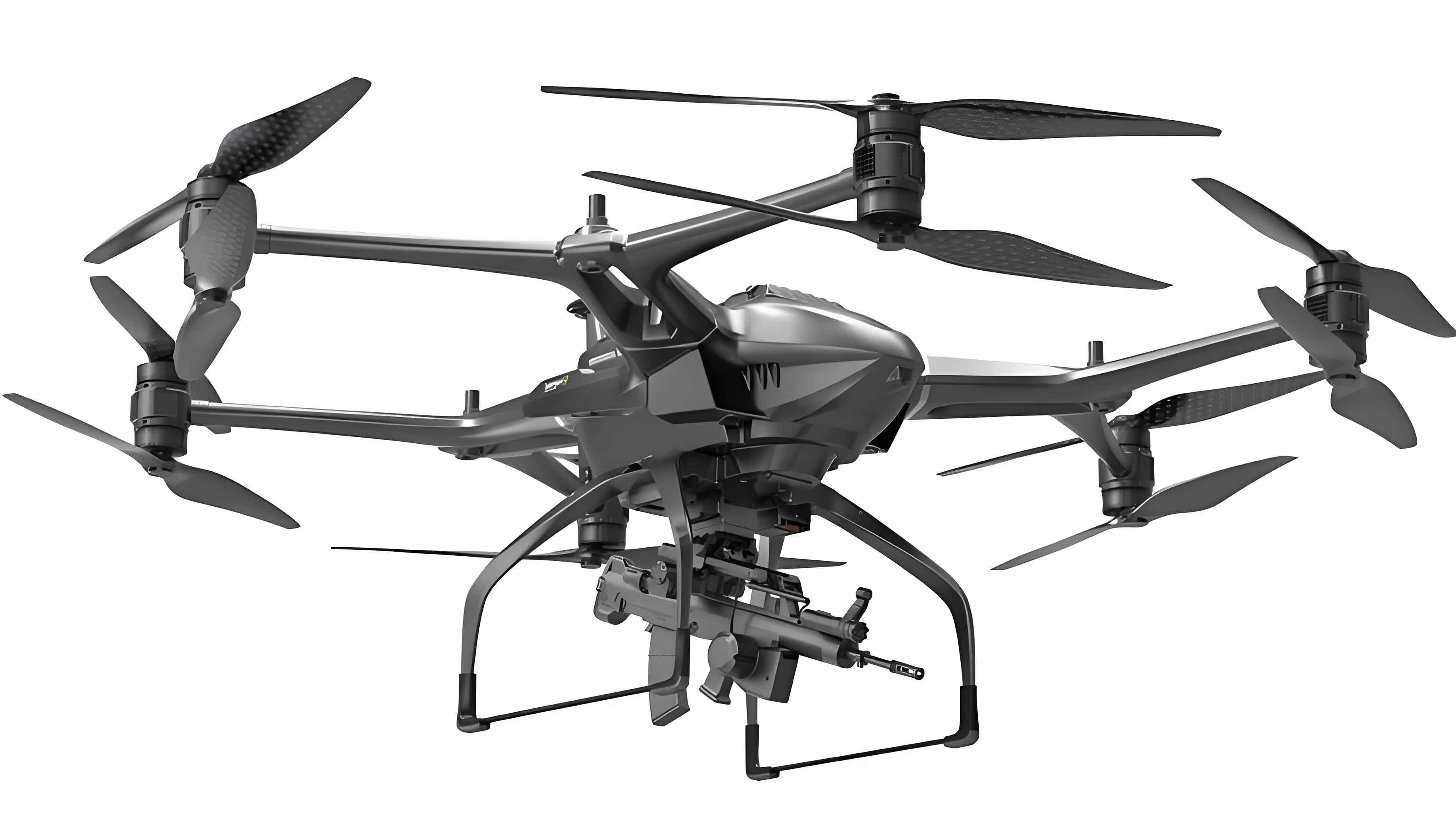
Future enhancements to this modeling approach are manifold. The feature set can be expanded to include technological sophistication indices, manufacturing complexity metrics, or the use of specific exotic materials, which are significant cost drivers for next-generation military drone systems. Furthermore, the SVR framework can be extended. $\nu$-SVR, an alternative formulation, allows the control of the number of support vectors and the width of the tube automatically. For programmatic risk analysis, one could explore the use of SVR in conjunction with Monte Carlo simulation, where distributions for input parameters (e.g., optimistic, pessimistic estimates for weight or speed) are sampled, and the SVR model generates a corresponding distribution of predicted costs.
Conclusion
The development of modern military drone systems demands sophisticated and reliable cost forecasting tools. This article has demonstrated that Support Vector Regression provides a powerful, theoretically sound framework for this task, particularly when historical data is limited. By effectively managing the trade-off between model complexity and empirical error through structural risk minimization, the SVR model achieved a higher prediction accuracy on a test case compared to traditional neural networks and linear regression. The methodology outlined—from feature selection based on engineering principles to the heuristic tuning of hyperparameters like $C$, $\epsilon$, and the RBF kernel’s $\gamma$—provides a practical roadmap for analysts. As the capabilities and roles of military drone platforms continue to expand, leveraging advanced, robust machine learning techniques like SVM will be indispensable for ensuring the financial viability and strategic success of these critical defense programs.