
1. Introduction and Research Background
The unmanned aerial vehicle (UAV) industry has become a critical domain for supporting the national strategy of building a leading aviation power and driving the iterative upgrading of aviation equipment. Current UAV research and development typically follows a conventional process involving document-based design, physical prototyping, testing, and iterative validation. However, this traditional workflow suffers from inadequate mechanisms for linking cyber and physical domains and faces significant difficulties in tracing parameter coordination, which severely constrains the efficiency of UAV system design and performance evaluation.
Within the context of low-altitude economy development, UAVs are now widely applied across various industrial sectors, including power grid inspection, agricultural plant protection, oil and gas pipeline monitoring, and aerial photography. Pipeline inspection, in particular, presents unique challenges due to the need for sustained flight stability, precise trajectory tracking, and reliable performance under adverse weather conditions. The limitations of traditional design approaches are primarily manifested in two aspects.
Figure 1 below illustrates the general application context of the proposed design framework in this research.
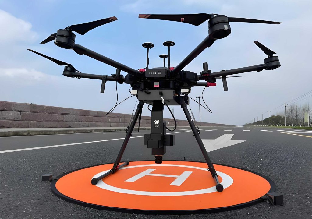
First, the traditional design process lacks a unified model to support collaborative cyber-physical domain modeling for specific application scenarios. The task logic and dynamic responses of UAV systems cannot be uniformly represented, hindering performance optimization and engineering implementation. Second, cyber-physical domain models in UAV design lack dynamic characterization mechanisms. Traditional design methods rely on manual, experience-based judgments and multiple rounds of physical prototype testing and iteration, which not only hinders the overall improvement of power coupling reliability but also delays the optimization of development efficiency.
To address these issues, this paper proposes an integrated design method for the full UAV inspection process. Based on the theory of Model-Based Systems Engineering (MBSE), this research aims to establish a full-lifecycle framework covering system modeling, implementation planning, collaborative control, and simulation verification. Taking pipeline inspection as a representative mission scenario, the proposed method achieves deep integration of cyber and physical domains through structured modeling from scheme design to physical implementation.
2. MBSE-Based Modeling Theory and Methodology
MBSE is a cross-domain technical approach that employs formalized models to support system behavior analysis, scheme design, performance evaluation, and verification confirmation. Compared with traditional document-based processes, MBSE models can comprehensively capture system behavioral logic, structural characteristics, functional relationships, and performance indicators while maintaining consistency and traceability across different perspectives.
2.1 MBSE Methodologies and Modeling Languages
Several mainstream MBSE methodologies exist, including the Harmony methodology, Object-Oriented Systems Engineering Method (OOSEM), and Object-Process Methodology (OPM). The Harmony methodology, developed by IBM for embedded complex system development, aligns well with UAV system design requirements. It employs a behavior-driven approach that identifies system functions from behaviors and decomposes functions into corresponding physical architectures through hierarchical refinement.
For modeling languages, the Systems Modeling Language (SysML) provides a standardized visual modeling framework. SysML has nine types of diagrammatic models, including use case diagrams, activity diagrams, state machine diagrams, block definition diagrams, internal block diagrams, requirement diagrams, and parametric diagrams. These diagrams support multi-disciplinary system expression in behavior analysis, structural design, and parameter constraints.
Table 2.1 compares several common MBSE modeling tools.
| Tool Name | Developer | Key Features |
|---|---|---|
| MWORKS.Sysbuilder | Suzhou Tongyuan Softcontrol Technology Co., Ltd. | Based on Harmony methodology, supports complex engineering system architecture design and model construction |
| IBM Rational Rhapsody | IBM | Full UML/SysML support, strong code generation capabilities |
| No Magic MagicDraw | No Magic | Comprehensive SysML modeling, simulation analysis capability |
| Sparx Systems Enterprise Architect | Sparx Systems | UML/SysML compatible, requirement and document management |
| PTC Integrity Modeler | PTC | Cross-disciplinary collaborative modeling, lifecycle management |
In this research, the MWORKS.Sysbuilder platform was selected for information-domain modeling due to its strong support for the Harmony methodology. For physical-domain modeling and simulation, the MWORKS.Sysplorer platform was utilized, which supports Modelica-based multi-physics modeling.
2.2 Multi-Physics Domain Modeling Principles
The Modelica language is an open-source, object-oriented, non-causal modeling language widely used for constructing and simulating complex multi-physics domain models. It enables the unified modeling and analysis of multi-disciplinary system models under a common framework through energy conservation principles. Standard Modelica libraries cover mechanical, electrical, hydraulic, control, and thermal domains, facilitating rapid model construction and system-level simulation.
Modular modeling decomposes the overall system into independent sub-modules based on its functions and structures. After completing sub-module modeling, these modules are combined into a complete model according to interface rules. Modelica components are typically composed of connectors and behavior descriptions, where potential variables and flow variables are defined to enable power flow transmission, thus achieving coupled modeling of multi-physics field systems.
3. Information-Domain Modeling of the UAV System
3.1 Mission Planning for UAV Pipeline Inspection
The inspection mission covers the pipeline segment between points A and B in the designated area. Before takeoff, the UAV performs sensor and communication equipment self-checks to ensure flight safety and mission completion. After completing the self-check, it establishes communication with the ground terminal. The operator sends inspection segment information to the UAV through the ground terminal. Upon receiving the mission, the UAV completes autonomous takeoff according to control module instructions and executes the inspection task along the pipeline based on the preset route.
The entire inspection process can be divided into three phases: initial preparation, autonomous inspection, and mission conclusion. The mission scenario defines key waypoints including the takeoff point C, image acquisition point D, inspection start point E, and inspection end point H. During the mission, the UAV maintains a specified safety distance from the pipeline while ensuring that the camera can accurately capture pipeline body and surrounding environment information.
3.2 System Information-Domain Architecture Analysis
According to the Harmony methodology, system analysis begins with identifying stakeholders. Pipeline operation enterprises represent the direct user group, primarily concerned with inspection efficiency and detection result accuracy. System designers focus on the engineering feasibility of mission behaviors and architecture extensibility, requiring clear understanding of flight control, mission payload, and communication link sub-systems. Maintenance personnel emphasize convenience of repair and component replacement.
Through behavioral analysis and system boundary determination, the primary stakeholders of the rotor UAV system were identified as ground control personnel and satellite systems. The system-level requirements for the UAV inspection mission were then systematically established, as shown in Table 3.1.
| ID | Requirement Name | Requirement Level |
|---|---|---|
| 0.1 | The rotor UAV shall have operational capability | Level 1 |
| 0.2 | The rotor UAV shall have cruising capability | Level 1 |
| 0.3 | The rotor UAV shall have emergency handling capability | Level 1 |
Based on the three primary requirements, the second-level requirement system was further refined as shown in Table 3.2, covering flight control, mission execution, and safety assurance capabilities.
| ID | Requirement Description | Requirement Level |
|---|---|---|
| 1.1 | The rotor UAV shall have mission preparation capability | Level 2 |
| 1.2 | The rotor UAV shall have takeoff capability | Level 2 |
| 1.3 | The rotor UAV shall have return-to-home capability | Level 2 |
| 1.4 | The rotor UAV shall have hovering capability | Level 2 |
| 1.5 | The rotor UAV shall have actuator response capability | Level 2 |
| 2.1 | The rotor UAV shall have relative positioning capability | Level 2 |
| 2.2 | The rotor UAV shall have command communication capability | Level 2 |
| 2.3 | The rotor UAV shall have detection capability | Level 2 |
| 2.4 | The rotor UAV shall have path planning capability | Level 2 |
| 2.5 | The rotor UAV shall have pipeline trajectory following capability | Level 2 |
| 3.1 | The rotor UAV shall have attitude anomaly handling capability | Level 2 |
| 3.2 | The rotor UAV shall have energy insufficiency handling capability | Level 2 |
3.3 Functional Analysis and Architecture Modeling
Using the SysML use case diagram, the functional activities of the UAV system were defined and organized hierarchically. The use case diagram, constructed with the pipeline inspection mission as the top-level objective, follows the stage evolution logic of the inspection process. The E, F, G, H waypoint nodes were simplified into system use cases with clear functional boundaries, and the specific functional activities were expanded through the include relationship «include» to achieve mapping from mission behaviors to system functional structures.
The behavioral logic of the inspection process was further defined using SysML activity diagrams. The activity diagram demonstrates that after the initial node publishes the mission, the system verifies that the UAV meets the execution conditions before entering the flight phase. The UAV sequentially executes climb, cruise, and descent operations. After reaching the predetermined mission altitude, the controller determines through feedback that the UAV has entered the inspection route and completes the inspection mission according to the flight path. After the flight route is completed, the decision node in the control system determines the completion status of the inspection mission.
For structural analysis, the UAV system was divided into functional modules, physical components, and software components. The internal block diagram depicts the composition and connections between sub-systems. The airframe serves as the physical carrier, with the flight control system as the core controller connected through standard interfaces to GPS satellite positioning, inertial measurement units (IMU), anemometers, and other sensing devices. The path planning module provides optimal flight routes and waypoint information to the flight control system, which then controls the servo motors to adjust rotor speeds to maintain attitude stability.
3.4 Mechanism Parameter Models
According to the behavior-structure-function-parameter principle of the Harmony methodology, the functional and logical architecture is mapped to specific physical parameter constraints. Parametric models were developed to provide unified description and verification of key UAV system mass parameters. The model uses total system mass constraint as the core, with constraint properties defining the relationship between total mass and component masses. Equation constraints associate sub-system mass parameters to ensure consistency and traceability between system-level mass indicators and component-level parameters.
The constraint expression for overall mass validation can be formulated as:
$$M_{total} = M_{fuselage} + M_{arm} + M_{rotor} + M_{motor} + M_{battery}$$
This method transforms design rules into computable model constraints and establishes a closed loop among parameter definition, constraint verification, and design decision-making. It provides early-stage parameter consistency analysis and feasibility assessment support for the UAV system design.
4. Multi-Physics Domain Modeling and Dynamic Response Analysis
4.1 Coordinate System Definition and Transformation
To accurately describe the spatial position and attitude changes of the UAV, two coordinate systems need to be defined. The inertial coordinate system E (oexeyeze) has its origin at a fixed ground point, with the x-axis pointing toward the geomagnetic north, the y-axis determined by the right-hand rule, and the z-axis opposite to gravity. The body coordinate system B (obxbybzb) has its origin at the UAV center of mass, with the x-axis along the UAV forward direction, the y-axis determined by the right-hand rule, and the z-axis pointing downward.
The transformation from the inertial coordinate system to the body coordinate system can be completed through three successive rotations. The rotation matrices are given by:
$$R(\phi) = \begin{bmatrix} 1 & 0 & 0 \\ 0 & \cos\phi & \sin\phi \\ 0 & -\sin\phi & \cos\phi \end{bmatrix}$$
$$R(\theta) = \begin{bmatrix} \cos\theta & 0 & -\sin\theta \\ 0 & 1 & 0 \\ \sin\theta & 0 & \cos\theta \end{bmatrix}$$
$$R(\varphi) = \begin{bmatrix} \cos\varphi & \sin\varphi & 0 \\ -\sin\varphi & \cos\varphi & 0 \\ 0 & 0 & 1 \end{bmatrix}$$
The overall transformation matrix from the inertial coordinate system to the body coordinate system is:
$$R_E^B = R(\phi)R(\theta)R(\varphi) = \begin{bmatrix} \cos\theta\cos\varphi & \cos\theta\sin\varphi & -\sin\theta \\ \sin\phi\sin\theta\cos\varphi – \cos\phi\sin\varphi & \sin\phi\sin\theta\sin\varphi + \cos\phi\cos\varphi & \sin\phi\cos\theta \\ \cos\phi\sin\theta\cos\varphi + \sin\phi\sin\varphi & \cos\phi\sin\theta\sin\varphi – \sin\phi\cos\varphi & \cos\phi\cos\theta \end{bmatrix}$$
4.2 UAV Dynamics Modeling
To facilitate the construction of the UAV dynamics model, the following assumptions were adopted:
(1) The quadrotor UAV is treated as an ideal rigid body with complete symmetry in both geometric structure and mass distribution.
(2) The UAV center of mass strictly coincides with the origin of the body coordinate system.
(3) All rotors and propellers are rigid components without elastic deformation.
(4) Ground interaction effects are neglected, considering only free-flight conditions.
(5) Higher-order nonlinear aerodynamic factors are neglected.
According to Newton’s laws, the resultant external force acting on the UAV includes the total thrust from the four rotors, gravity, and aerodynamic drag:
$$\sum F = F_B^E + F_g + F_f$$
For each rotor, the thrust is proportional to the square of the rotor speed:
$$F_i = C_L N_i^2, \quad i = 1,2,3,4$$
where $C_L$ is the lift coefficient and $N_i$ is the rotational speed of the i-th motor. The total thrust in the body coordinate system is transformed to the inertial coordinate system using the rotation matrix:
$$F_B^E = R_B^E \begin{bmatrix} 0 \\ 0 \\ \sum_{i=1}^{4} F_i \end{bmatrix}$$
The gravitational force is $F_g = [0, 0, -mg]^T$, and the aerodynamic drag can be expressed as $F_f = [-K_x\dot{x}, -K_y\dot{y}, -K_z\dot{z}]^T$. Combining these terms, the translational equations of motion are:
$$\ddot{x} = \frac{(\cos\phi\sin\theta\cos\varphi + \sin\phi\sin\varphi)F_B}{m} – \frac{K_x\dot{x}}{m}$$
$$\ddot{y} = \frac{(\cos\phi\sin\theta\sin\varphi – \sin\phi\cos\varphi)F_B}{m} – \frac{K_y\dot{y}}{m}$$
$$\ddot{z} = \frac{\cos\phi\cos\theta F_B}{m} – g – \frac{K_z\dot{z}}{m}$$
For rotational motion, the total torque consists of rotor torque, gyroscopic torque, and drag torque. The rotor torque components are determined by the differential thrust forces:
$$M_\phi = (F_4 – F_2)L$$
$$M_\theta = (F_3 – F_1)L$$
$$M_\varphi = d(N_1^2 – N_2^2 + N_3^2 – N_4^2)$$
where $L$ is the distance from the propeller center to the UAV center of mass and $d$ is the drag coefficient. The rotational equations are:
$$\dot{\omega}_x = \frac{I_y – I_z}{I_x}\omega_y\omega_z + \frac{(F_4 – F_2)L – K_\phi\omega_x + J_r\omega_y N}{I_x}$$
$$\dot{\omega}_y = \frac{I_z – I_x}{I_y}\omega_x\omega_z + \frac{(F_3 – F_1)L – K_\theta\omega_y – J_r\omega_x N}{I_y}$$
$$\dot{\omega}_z = \frac{I_x – I_y}{I_z}\omega_x\omega_y + \frac{d(F_1 – F_2 + F_3 – F_4) – K_\varphi\omega_z}{I_z}$$
Table 4.1 lists the key parameters of the UAV used in this study.
| Parameter | Symbol | Value | Unit |
|---|---|---|---|
| Mass | m | 1.25 | kg |
| Arm length | l | 0.38 | m |
| Rotor radius | R | 0.16 | m |
| Rotor inertia | Jr | 1 | kg·m² |
| Roll moment of inertia | Ix | 0.096 | kg·m² |
| Pitch moment of inertia | Iy | 0.096 | kg·m² |
| Yaw moment of inertia | Iz | 0.016 | kg·m² |
4.3 Wind Disturbance Environment Modeling
The wind disturbance environment was modeled by combining mean wind and turbulent wind components. The mean wind varies slowly with time and represents the background wind field. It was expressed as:
$$\bar{v}(h) = W_{href} \times \frac{\ln(h/z_0)}{\ln(h_{ref}/z_0)}$$
where $z_0$ represents the surface roughness height, $h$ is the current flight altitude, $W_{href}$ is the wind speed at reference height, and $h_{ref}$ is the reference height.
For turbulent wind modeling, the Dryden spectral model was selected due to its simple structure and computational efficiency. The power spectral density functions of turbulent velocity components along the body coordinate system are:
$$\Phi_u(\omega) = \frac{\sigma_u^2 L_u}{\pi V} \cdot \frac{1}{1 + (L_u \omega/V)^2}$$
$$\Phi_v(\omega) = \frac{\sigma_v^2 L_v}{\pi V} \cdot \frac{1 + 12(L_v \omega/V)^2}{1 + 4(L_v \omega/V)^2}$$
$$\Phi_w(\omega) = \frac{\sigma_w^2 L_w}{\pi V} \cdot \frac{1 + 12(L_w \omega/V)^2}{1 + 4(L_w \omega/V)^2}$$
For low-altitude UAV operations, the turbulence scale and intensity can be characterized as:
$$L_w = 2h$$
$$L_u = L_v = h(0.177 + 0.000823h)^{1.2}$$
$$\sigma_w = 0.1W_{href}$$
$$\sigma_u = \sigma_v = \sigma_w(0.177 + 0.000823h)^{0.4}$$
The shaping filters for generating turbulent wind components from white noise inputs are:
$$H_u(s) = \frac{\sigma_u}{V^{1/2}} \cdot \frac{L_u}{1 + (L_u/V)s}$$
$$H_v(s) = \frac{\sigma_v}{V^{1/2}} \cdot \frac{L_v(1 + \sqrt{12}(L_v/V)s)}{(1 + (2L_v/V)s)^2}$$
$$H_w(s) = \frac{\sigma_w}{V^{1/2}} \cdot \frac{L_w(1 + \sqrt{12}(L_w/V)s)}{(1 + (2L_w/V)s)^2}$$
The total wind field was obtained by superposition:
$$V_{xx} = \bar{v}_{xx} + u_d, \quad V_{yy} = \bar{v}_{yy} + v_d, \quad V_{zz} = \bar{v}_{zz} + w_d$$
4.4 Control System Modeling
The control system was designed as a combination of Line-of-Sight (LOS) trajectory tracking and PID control. The LOS method introduces a virtual line of sight between the UAV position and the target trajectory. The desired heading angle is calculated based on the lateral deviation $e_y$ and a look-ahead distance parameter $\Delta$:
$$\varphi_d = \varphi_p – \arctan\left(\frac{e_y}{\Delta}\right)$$
where $\varphi_d$ is the desired track angle and $\varphi_p$ is the current track heading angle. The PID control law was formulated as:
$$u(t) = K_p e(t) + K_i \int_0^t e(\tau)d\tau + K_d \frac{de(t)}{dt}$$
The integrated control strategy combines LOS trajectory tracking with PID attitude control. The process follows these steps: generating waypoint sequences from the preset inspection path, computing lateral deviation from the target trajectory, calculating the desired heading angle using the LOS algorithm, feeding this into the PID controller to generate control outputs, adjusting the UAV attitude to converge toward the target trajectory, and automatically switching to the next waypoint when the current one is within the decision radius.
5. Simulation and Dynamic Response Analysis
5.1 Simulation Configuration
Based on the Modelica language and the MWORKS platform, the complete UAV dynamics model was established through bottom-up system integration. The model includes coordinate transformation, body dynamics, control system, and environmental system components. The generalized Kirchhoff network approach was adopted for cross-domain coupled sub-system co-simulation. When configuring the simulation, careful attention was paid to interface parameter consistency and matching among sub-systems.
5.2 Dynamic Response under No-Wind Conditions
The attitude angle variations during the inspection mission under no-wind conditions show that during the initial 0-10 s phase, both roll and pitch angles exhibit transient fluctuations of approximately 0.25 rad amplitude, converging rapidly to near-zero within 5-8 s. This indicates good initial convergence and damping characteristics of the multi-physics model. During steady inspection flight, attitude angles vary within small ranges, with roll and pitch steady-state errors close to zero. The yaw angle changes slowly, showing a 0.12 rad initial deviation that gradually converges exponentially.
The velocity component responses show that during initial takeoff and transient establishment, x-axis velocity reaches a peak of 5 m/s, y-axis velocity peaks at 4 m/s, and z-axis velocity remains below 1 m/s. During stable cruise, x-axis velocity stabilizes near 3 m/s with small fluctuation amplitude, while y-axis and z-axis velocities remain essentially near zero. The simulation results demonstrate that the multi-physics model exhibits excellent velocity regulation and dynamic stability.
5.3 Dynamic Response under Wind Disturbance Conditions
With wind disturbance applied, the attitude angle responses show more significant fluctuations. The roll angle reaches a maximum of 0.25 rad, and the pitch angle reaches 0.3 rad during the initial phase. Due to the attitude controller, these deviations decay rapidly within 10 s. During the mid-mission phase of 60-80 s, pitch angle fluctuation amplitude is largest, reaching a peak near -0.35 rad, while roll angle fluctuates around -0.25 rad. This indicates that pitch angle is more sensitive to external disturbances, reflecting the significant impact of longitudinal aerodynamic disturbances on attitude stability during low-altitude inspection.
The yaw angle shows a step-like change, transitioning from 0.12 rad to 0.25 rad with stable convergence and no obvious overshoot. Despite substantial transient deviations under strong wind disturbance, all attitude variables remain bounded and recover to stable states within 10-15 s after disturbance subsides. Compared with no-wind conditions, the peak amplitudes of roll and pitch angles increase to approximately 0.3 rad and stabilization time extends to 10-15 s, yet the system maintains zero steady-state error and bounded responses.
The velocity responses under wind disturbance show that the x-axis velocity establishes forward cruise speed with a transient peak of 5.5 m/s and converges to 3 m/s. During the mid-mission phase, the x-axis velocity reverses with a minimum value near -8 m/s, recovering within 10-15 s. The y-axis velocity shows oscillatory responses peaking at 4 m/s, while the z-axis velocity remains near zero throughout. The comparative analysis confirms that despite external disturbances affecting dynamic responses, the designed control strategy effectively suppresses disturbance interference.
6. Integrated Simulation for the Full Inspection Process
6.1 Cyber-Physical Domain Co-Simulation Framework
The joint simulation framework integrates the information-domain model with the physical-domain model. The information-domain model describes the decision logic and mission states during the UAV inspection process, using mission publication as the starting point. The UAV sequentially completes state determination, takeoff control, trajectory flight, and inspection photography behaviors. During the co-simulation, the Modelica dynamics model continuously provides flight state information to the activity diagram for mission logic judgment and subsequent action decisions. According to the inspection mission behaviors, real-time determination of UAV operating states is performed, and control commands including takeoff control, inspection flight, and hover photography are sent to the dynamics model.
6.2 Mission Analysis and Scenario Design
In complex terrain conditions, the rotor UAV pipeline inspection mission evolves into a complex mission process integrating continuous state evolution and discrete mission triggering. The UAV state vector is defined as:
$$Z(t) = [X(t), V(t), \Theta(t), \omega(t)]^T$$
where $X(t)$ denotes position, $V(t)$ indicates velocity, $\Theta(t)$ represents attitude angles, and $\omega(t)$ denotes angular velocities. The continuous dynamics process is expressed as:
$$\dot{Z}(t) = f(Z(t), U(t))$$
For describing the spatial characteristics of pipeline inspection, the mission function is formulated as:
$$J_{task} = \omega_\Gamma \int_0^S \delta_\Gamma(X(s))ds + \sum_{i=1}^{N_T} \omega_i \delta_i(X(t) – P_i)$$
where the first term covers continuous flight coverage requirements and the second term represents discrete event triggering mechanisms at key target positions. For the inspection scenario, the mountain terrain model was decomposed into smooth terrain, non-smooth terrain, and ridge/valley features:
$$h(x,y) = h_s(x,y) + h_c(x,y) + h_r(x,y)$$
The smooth terrain was modeled using superimposed trigonometric functions:
$$h_s(x,y) = a\sin(y) + b\sin(x) + c\cos(x,y) + d\cos(y) + e\sin(x,y) + f\sin(y)$$
where parameters $a$ through $g$ control terrain amplitude and spatial frequency at different scales. Cliff terrain was represented using level set functions with smooth approximation, and ridge/valley features were described using Gaussian-type smoothing functions along defined centerlines.
6.3 Full-Process Simulation Results and Verification
In the xoy plane trajectory, the UAV exhibits initial lateral adjustment and oscillation, after which the trajectory stabilizes to maintain a fixed lateral offset of 5 m along the inspection direction. During the mid-section inspection, small y-direction deviations demonstrate effective horizontal control, consistent with pipeline inspection requirements for consistency and continuity. At the position approaching the inspection end, horizontal displacement and direction adjustment occur, with trajectory continuity confirming that the mission and planning scheme maintains continuous dynamic response without trajectory mutation.
In the xoz plane, the flight altitude rapidly increases during the initial phase, undergoes slight adjustment at a horizontal distance of approximately 10 m, then maintains the preset inspection altitude. During the inspection segment, the altitude remains essentially stable at 2.25 m, demonstrating that vertical control effectively resists external disturbance effects. At mission transition positions, the altitude changes to 3.25 m, reflecting the UAV performing altitude adjustment at critical mission nodes.
The three-dimensional trajectory in the inertial coordinate system exhibits piecewise smooth characteristics with local adjustments. Along the inspection segment, the flight path is stable and continuous. Near the starting phase and the inspection end, trajectory spatial turns and altitude changes occur. The simulation results confirm that the proposed inspection mission description and planning method achieves effective coupling between flight dynamics and discrete missions in three-dimensional space.
6.4 Control Response Analysis
The altitude response curve demonstrates the operation of the altitude controller at different time periods. The UAV takes off from the ground and completes target altitude adjustment within a short period. Although the altitude exhibits obvious fluctuations in the early takeoff phase, it stabilizes at 2.25 m under controller action. During the 150 m inspection phase, the altitude remains essentially at 2.25 m, verifying that the altitude control module effectively suppresses external disturbances and system dynamic coupling. At approximately 150 m, the UAV receives mission commands for altitude adjustment. The altitude shows brief descent followed by rapid rise, stabilizing at 3.25 m. The altitude response exhibits slight oscillatory decay characteristics and completes stable convergence within a short period.
The pitch angle variation represents the attitude control module’s regulation capability. When transitioning from static state to flight, the pitch angle instantaneously increases to 3 rad due to coupling effects during takeoff, but rapidly converges and stabilizes under the control system. At approximately 150 m flight distance, during mission adjustment, the attitude angle oscillates briefly before quickly recovering and reconverging to a stable state. The results indicate that the designed attitude control system effectively suppresses attitude disturbances and maintains stable flight attitude.
Table 6.1 summarizes the key performance metrics observed across the simulation scenarios.
| Metric | No-Wind Condition | Wind Disturbance Condition |
|---|---|---|
| Initial attitude peak | 0.25 rad | 0.30 rad |
| Attitude stabilization time | 5-8 s | 10-15 s |
| X-axis speed peak | 5 m/s | 5.5 m/s |
| Cruise speed | 3 m/s | 3 m/s |
| Altitude stability | ±0.05 m | ±0.10 m |
| Maximum pitch deviation | 0.15 rad | 0.35 rad |
| Steady-state error | Zero | Zero |
7. Conclusions and Future Work
This research proposed an integrated design method for the full UAV inspection process based on MBSE principles. The method establishes a comprehensive design framework that integrates system modeling, implementation planning, collaborative control, and simulation verification. Through the unified modeling of information-domain and physical-domain models, the proposed method addresses the critical limitations of traditional UAV design approaches.
The main contributions of this work are summarized as follows.
(1) An information-domain architecture model for the UAV inspection process was established following the MBSE methodology. This model integrates behavioral, functional, structural, and parametric views, providing a unified foundation for system design and validation. The structured modeling approach enables traceable mapping from mission requirements to system architecture, ensuring consistency between system-level objectives and detailed subsystem design parameters.
(2) A multi-physics domain simulation model was developed based on the information-domain architecture. The model incorporates UAV body dynamics, wind disturbance environments, and control systems within a unified modeling framework. Dynamic response analysis under both no-wind and wind disturbance conditions validated the model accuracy and effectiveness in predicting UAV motion responses under different environmental conditions.
(3) A cyber-physical domain co-simulation framework was established for the full inspection process verification. Through the integration of the information-domain model and physical-domain model in the MWORKS platform, the complete inspection mission was simulated and validated. The simulation results confirmed the feasibility of the proposed design method, providing a digital support path for UAV system solutions.
The innovation points of this research are as follows:
(1) A unified modeling scheme based on MBSE was proposed to address the inadequate cyber-physical domain association mechanisms in traditional UAV development. This scheme realizes full-chain mapping from system behavior, functional logic, and physical prototypes, revealing the coupling mechanisms between UAV behaviors and sub-systems.
(2) An integrated design methodology for the full UAV inspection process was established by constructing a cyber-physical domain optimization model supporting parameter mapping and consistent operating conditions. This methodology forms a closed-loop dynamic verification system covering scenario-driven design, model generation, and simulation validation.
Future research directions include:
(1) Introducing more complex environmental factors and operational constraints to enhance the model’s fidelity in representing real inspection scenarios. System-level models can be combined with local high-fidelity models to achieve multi-resolution co-simulation.
(2) Extending the closed-loop framework by incorporating optimization algorithms and intelligent decision-making methods. Simulation results can be used not only for verifying system design rationality but also for automatically optimizing system parameters and control strategies.
(3) Integrating hardware-in-the-loop simulation and actual flight tests to establish closer connections between system models and real UAV flight data. This will further verify the applicability and robustness of the proposed method in engineering practice.