
The artistic and commercial demand for large-scale, coordinated aerial displays has propelled the development of sophisticated formation drone light show systems. These systems involve hundreds, sometimes thousands, of UAVs operating synchronously to create dynamic, illuminated patterns in the night sky. A core challenge in orchestrating such a spectacle is not just the initial planning of the grand animation, but the dynamic and safe reorganization of the fleet’s flight paths—its formation drone light show structure—during transitions, in response to contingencies, or for multi-part performances. This article presents a comprehensive methodology for the real-time path reconstruction of a formation drone light show fleet, integrating multi-task execution planning with a time-varying vector field control strategy.
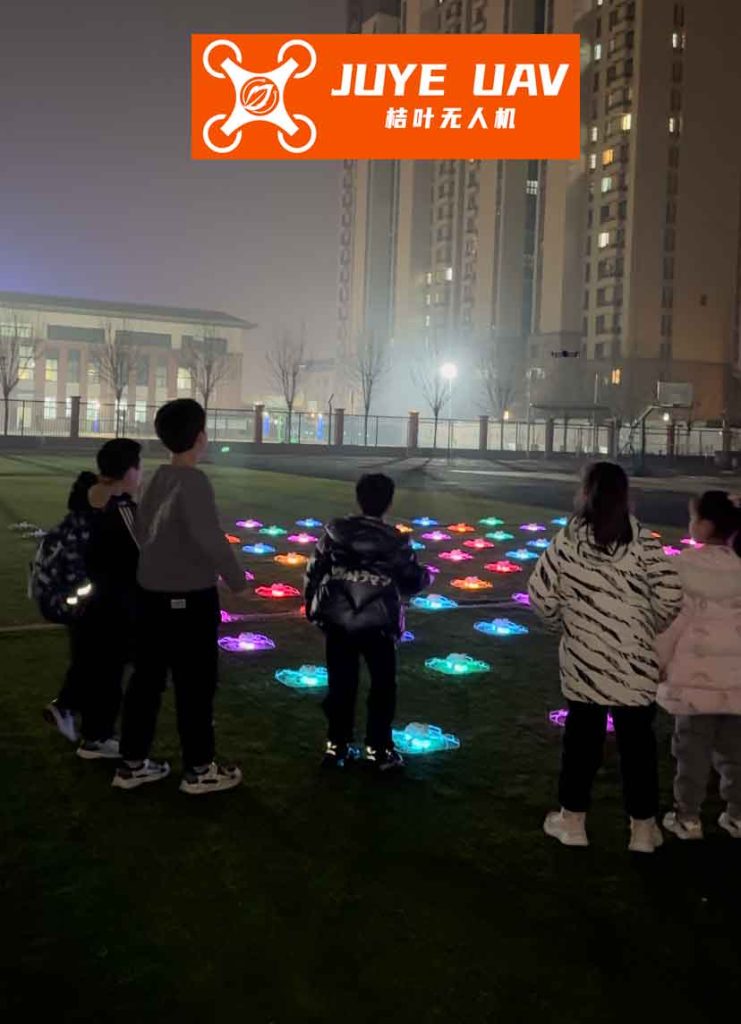
The foundation of a reliable formation drone light show lies in its system architecture and the initial task planning. A typical fleet consists of multiple homogeneous drones, a central ground control station (GCS) for high-level command, and a local inter-drone communication network. For a complex show divided into several sequential acts or “scenes,” each drone must be assigned a specific trajectory—a series of waypoints and maneuvers—for each act. This is the multi-task execution plan.
Let us define the complete performance plan for a single drone $D_i$ as an ordered sequence of $K$ show segments or acts:
$$ \text{Plan}_i = \{ \text{Act}^{(i)}_1, \text{Act}^{(i)}_2, …, \text{Act}^{(i)}_K \} $$
where each act $\text{Act}^{(i)}_k$ for drone $D_i$ is defined by the target pattern position it must achieve and the specific flight route to get there: $\text{Act}^{(i)}_k = \{ \text{Target}_{j}, \text{Route}^{(i)}_k \}$. The goal of the planning algorithm is to assign these acts to all $N$ drones in the formation drone light show to optimize overall performance metrics. Two primary, often conflicting, objectives are considered:
- Minimize Total Fleet Travel Distance: This reduces overall energy consumption, a critical factor for battery-operated show drones.
- Minimize Total Show Duration: This is dictated by the drone with the longest cumulative flight path, ensuring the show’s pacing is efficient.
We formulate a composite objective function $J$ to balance these goals during the planning phase for the formation drone light show:
$$ \text{Min } J = \omega_1 \cdot \max_{i \in [1, N]} (L_i) + \omega_2 \cdot \frac{\sum_{i=1}^{N} L_i}{N} $$
where $L_i = \sum_{k=1}^{K} \text{Length}(\text{Route}^{(i)}_k)$ is the total path length for drone $D_i$, and $\omega_1$, $\omega_2$ are weighting coefficients reflecting the priority of time versus energy efficiency for this particular formation drone light show.
| Parameter | Symbol | Typical Value / Range | Description |
|---|---|---|---|
| Number of Drones | $N$ | 100 – 2000 | Fleet size for the light show. |
| Show Duration | $T_{total}$ | 5 – 20 min | Total planned performance time. |
| Drone Max Speed | $v_{max}$ | 10 m/s | Maximum operational airspeed. |
| Safety Distance | $d_{safe}$ | 1.5 – 3 m | Minimum inter-drone separation. |
| Time Weight | $\omega_1$ | 0.6 – 0.8 | Priority for synchronized timing. |
| Energy Weight | $\omega_2$ | 0.2 – 0.4 | Priority for battery conservation. |
Once the high-level plan is set, the real-time control challenge begins. Each drone in the formation drone light show is equipped with a hierarchical, autonomous control framework. This framework processes global commands, assesses local neighbor states via communication, and makes micro-level navigation decisions to follow its assigned path while avoiding collisions. The key innovation for smooth path following and dynamic reconstruction lies in the use of a Time-Varying Vector Field.
Consider a drone needing to follow a curved path, which can be approximated by a segment of a moving circle. Let $\vec{r}(t)$ be the vector from the circle’s instantaneous center $O(t)$ to the drone’s position, with magnitude $r(t) = |\vec{r}(t)|$. The desired path is defined by a circle of radius $R(t)$. We construct a guiding vector field $\vec{f}(\vec{r}, t)$ that directs the drone. The field consists of two components: a convergence component perpendicular to the path that pulls the drone toward the desired circle, and a propagation component tangent to the path that moves it along the trajectory.
Let $\hat{r}_{\parallel}$ be the unit vector parallel to $\vec{r}(t)$, and $\hat{r}_{\perp}$ be the orthogonal unit vector pointing in the desired direction of travel along the path. The vector field is designed as:
$$ \vec{f}(\vec{r}, t) = \frac{-\big( (r(t) – R(t)) – \lambda_2 \big) \hat{r}_{\parallel} + \lambda_1 \hat{r}_{\perp}}{\chi(\vec{r}, t)} $$
Here, $\lambda_1$ and $\lambda_2$ are control gains that adjust the aggressiveness of path following and convergence. The denominator $\chi(\vec{r}, t)$ is a scaling function set to ensure the magnitude of the desired velocity command equals a speed $v_d(t)$:
$$ \chi(\vec{r}, t) = \frac{\sqrt{ \big( (r(t) – R(t)) – \lambda_2 \big)^2 + \lambda_1^2 }}{v_d(t)} $$
The desired speed $v_d(t)$ is not constant. To ensure the entire formation drone light show reconstructs its pattern synchronously at a predefined future time $t_f$, each drone adjusts its speed based on its estimated time of arrival. If a drone is predicted to arrive early ($\hat{t}_{arrival} < t_f$), it slows down; if late, it speeds up:
$$ v_d(t) = v_{nominal} + k_T (t_f – \hat{t}_{arrival}(t)) $$
where $k_T > 0$ is a control gain. The estimated arrival time $\hat{t}_{arrival}$ is continuously recalculated based on remaining path length, which may involve $n$ circular arc segments. For an arc segment with time-varying curvature $\eta(t)$ and radius $R(t)$, the arrival time derivative is:
$$ \frac{d \hat{t}_{arrival}}{dt} \propto \frac{n^*}{\,v_d(t)\,} \left( \dot{R}(t) \eta(t) + R(t) \dot{\eta}(t) \right) $$
where $n^*$ is the number of remaining arcs. To drive $\hat{t}_{arrival} \rightarrow t_f$, we can dynamically adjust the path geometry itself, specifically the arc angle $\eta(t)$, using a simple control law:
$$ \dot{\eta}(t) = -\lambda_3 (\hat{t}_{arrival} – t_f) $$
with $\lambda_3 > 0$. This elegant solution means the path is not static; it reconstructs itself in real-time via the time-varying vector field parameters to guarantee timely arrival for the formation drone light show sequence. The drone’s desired heading $\psi_d$ is derived from the vector field:
$$ \psi_d(t) = \arctan\left( \frac{ -\big((r-R)+\lambda_2\big)(y-y_o) \pm \lambda_1 (x-x_o) }{ -\big((r-R)+\lambda_2\big)(x-x_o) \mp \lambda_1 (y-y_o) } \right) $$
where $(x, y)$ is the drone’s position and $(x_o, y_o)$ is the moving center $O(t)$.
| Parameter | Symbol | Role in Path Reconstruction |
|---|---|---|
| Path Radius | $R(t)$ | Defines the curvature of the desired flight path segment; can be varied for dynamic morphing. |
| Arc Angle | $\eta(t)$ | Defines the length of the curved path; actively adjusted to synchronize arrival times. |
| Convergence Gain | $\lambda_1$ | Controls how tightly the drone follows the tangent of the path. |
| Offset Gain | $\lambda_2$ | Allows for a stable offset from the nominal path if needed for spacing. |
| Synchronization Gain | $\lambda_3$ | Governs the rate at which the path geometry adapts to meet the global timing constraint. |
| Speed Adjustment Gain | $k_T$ | Determines how aggressively speed is corrected based on arrival time error. |
Safety is paramount in a dense formation drone light show. The vector field framework integrates collision avoidance as a repulsive vector field component. When another drone enters a protected zone around a given drone, a repulsive term $\vec{f}_{rep}$ is added to the total guiding field $\vec{f}_{total} = \vec{f} + \vec{f}_{rep}$. This term pushes the drone away from the intruder, with magnitude inversely proportional to the square of the distance, ensuring smooth evasion without abrupt maneuvers that could disrupt the overall formation drone light show aesthetics.
For reconstruction scenarios—such as transitioning from a “star” pattern to a “globe” pattern—the multi-task plan provides the target states for each drone at the end of the transition. The time-varying vector field controller for each drone is then configured with the new target path parameters ($R(t_f)$, $\eta(t_f)$). The dynamic adjustment of $\eta(t)$ and $v_d(t)$ ensures all drones leave their old positions and converge onto their new positions in the reconstructed pattern simultaneously and safely, creating a seamless visual transformation for the audience.
In summary, the synergy of multi-task execution planning and time-varying vector field control creates a robust and flexible system for managing a formation drone light show. The planning stage optimally assigns complex aerial choreography, while the vector field controller enables precise, safe, and synchronized path following and dynamic reconstruction in real-time. This approach ensures the spectacular visual performance is not only beautiful but also intelligent and resilient.
| Metric | Traditional Waypoint Following | Static Vector Field Guidance | Proposed Time-Varying Vector Field |
|---|---|---|---|
| Synchronization Error | High (independent tracking) | Medium (no temporal adaptation) | Low (active path & speed adjustment) |
| Total Fleet Energy Use | High (inefficient paths) | Medium | Low (optimized plan + efficient tracking) |
| Collision Safety | Reactive only | Integrated but static | Proactive & Adaptive |
| Reconstruction Smoothness | Abrupt, segmented | Smooth but potentially mis-timed | Seamless & Synchronized |
| Suitability for Complex Formation Drone Light Show | Poor | Moderate | Excellent |