
In this research, I investigate the problem of global path planning for **unmanned aerial vehicles** in two typical complex low‑altitude environments: mountainous areas with continuous elevation surfaces and dense peak obstacles, and urban areas with dense regular building clusters. The core challenge is to generate a safe, smooth, and cost‑effective flight trajectory while respecting constraints such as minimum flight altitude, maximum turning angle, and path length. To address these challenges, I develop two multi‑strategy improved swarm intelligence optimization algorithms—an improved Hippopotamus Optimization (DMHO) and an improved Honey Badger Algorithm (MIHBA)—and validate their performance through benchmark tests, simulated three‑dimensional environment experiments, and real‑flight deployment on a custom quadrotor platform.
The remainder of this paper is organized as follows. Section 2 describes the environmental modeling and objective function. Section 3 presents the proposed DMHO algorithm and its application to mountainous path planning. Section 4 presents the proposed MIHBA algorithm and its application to urban path planning. Section 5 describes hardware experiments and validation. Section 6 concludes the paper and discusses future directions.
1. Environmental Modeling and Objective Function
The three‑dimensional flight space for **unmanned aerial vehicles** is defined as:
\[
\left\{ \left( x,y,z \right) \,|\, 0 \le x \le x_{\max},\; 0 \le y \le y_{\max},\; 0 \le z \le z_{\max} \right\}.
\]
I use a regular grid digital elevation model (DEM) to represent mountainous terrain. The elevation at any point \((x,y)\) is described by a continuous function \(z = f(x,y)\). For urban environments, I model buildings as rectangular or cylindrical obstacles with given center positions, widths, lengths, and heights.
The path cost function is formulated as:
\[
C = \sum_{i=1}^{n} \left( \omega_1 l_i + \omega_2 h_i + \omega_3 g_i \right),
\]
where \(l_i\) is the Euclidean length of segment \(i\), \(h_i\) is the altitude above ground, \(g_i\) is the threat index, and \(\omega_1,\omega_2,\omega_3\) are weight coefficients with \(\omega_1+\omega_2+\omega_3=1\).
Additional constraints include:
– Minimum flight altitude: \(H_i \ge H_{\min}\) for every segment \(i\).
– Minimum path segment length: \(l_i \ge l_{\min}\).
– Maximum turning angle: \(\cos\phi \le \frac{\mathbf{a}_i \cdot \mathbf{a}_{i+1}}{\|\mathbf{a}_i\| \|\mathbf{a}_{i+1}\|}\), where \(\mathbf{a}_i\) is the horizontal projection of segment \(i\).
– Maximum climb/dive angle: \(\tan\theta \le \frac{|z_i – z_{i-1}|}{\|a_i\|}\).
– Total path length: \(\sum_{i=1}^{n} l_i \le L_{\max}\).
2. Improved Hippopotamus Optimization Algorithm (DMHO) for Mountainous Terrain
The original Hippopotamus Optimization (HO) algorithm simulates the social behavior of hippopotamuses, including position updating, defense against predators, and escape behavior. However, HO suffers from premature convergence and low solution accuracy in complex high‑dimensional problems. To overcome these limitations, I propose DMHO with four improvement strategies.
2.1 Lévy Flight Initialization
Instead of uniform random initialization, I use Lévy flight to generate the initial population:
\[
X_i = X_{\min} + \mathrm{Levy}(\lambda) \cdot (X_{\max} – X_{\min}),
\]
where \(\mathrm{Levy}(\lambda)\) is a random step drawn from a Lévy distribution, enhancing population diversity and global exploration capability.
2.2 Dynamic Growth Ratio Mechanism
The original convergence factor \(T = \exp(-t/T_{\max})\) is replaced by a dynamic ratio based on the fitness of each individual:
\[
T_{\text{dyn}} = \frac{f_{\text{best}}}{f(i)},
\]
where \(f_{\text{best}}\) is the current best fitness and \(f(i)\) is the fitness of the \(i\)-th individual. This adaptive mechanism allows individuals with better fitness to explore further away from the mother group, leading to a more efficient search.
The position update of female and juvenile hippopotamuses is then modified as:
\[
X_i^{FB} = \begin{cases}
x_{ij} + h_1 \cdot D_{\text{hippo}} \cdot I_2 – MG_i, & \text{if } T_{\text{dyn}} > 1, \\
X_i^{FB}, & \text{otherwise}.
\end{cases}
\]
2.3 Adaptive Lens Opposition-Based Learning
Lens opposition-based learning (LOBL) uses the principle of convex lens imaging to generate a candidate opposite solution. The dynamic scaling factor \(k\) is defined as:
\[
k = \left( 1 + \left( t / T_{\max} \right)^{1/2} \right)^{10}.
\]
The opposite position is computed by:
\[
X_{\text{opp}} = \frac{lb+ub}{2} + \frac{lb+ub}{2k} – \frac{X_c}{k},
\]
where \(lb\) and \(ub\) are the lower and upper bounds of the search space, and \(X_c\) is the current individual. This strategy helps the algorithm escape from local optima.
2.4 Random Diffusion
To simulate the escape behavior when a hippopotamus encounters a group of predators, I introduce a random diffusion step:
\[
s = 0.1 \cdot R(1,d) \cdot (u_b – l_b),
\]
\[
X_i^{(t+1)} = X_i^{(t)} + s,
\]
where \(R(1,d)\) is a random vector of dimension \(d\) with elements between 0 and 1, and \(u_b,l_b\) are upper and lower bounds. This mechanism increases the exploration ability of the algorithm.
2.5 Benchmark Experiments
I evaluate DMHO on the 23 CEC2005 benchmark functions. The population size is set to 30 and the maximum number of iterations to 500. Each algorithm runs 50 independent trials. Table 1 presents the mean and standard deviation of DMHO and eight other algorithms (DBO, FHO, GSA, GWO, HBA, HHO, PSO, HO) for the unimodal functions \(f_1\)–\(f_7\).
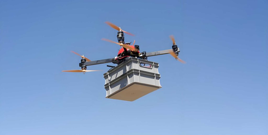
**Table 1: Mean and standard deviation comparisons on unimodal functions.**
| Func. | Algorithm | Mean | Std |
|——-|———–|——|—–|
| \(f_1\) | DBO | 9.3731E-111 | 6.1713E-110 |
| | FHO | 6.4786E-73 | 4.5192E-72 |
| | GSA | 1.4475E-233 | 0.0000E+00 |
| | GWO | 1.4928E-27 | 2.2817E-27 |
| | HBA | 8.6271E-134 | 5.1515E-133 |
| | HHO | 3.1486E-96 | 1.5311E-95 |
| | PSO | 2.3009E+00 | 1.0362E+00 |
| | HO | 0.0000E+00 | 0.0000E+00 |
| | **DMHO** | **0.0000E+00** | **0.0000E+00** |
| \(f_2\) | DBO | 5.7652E-55 | 3.4814E-54 |
| | FHO | 8.5438E-19 | 3.0567E-18 |
| | GSA | 1.5474E-111 | 1.0788E-110 |
| | GWO | 1.0765E-16 | 1.4063E-16 |
| | HBA | 2.7662E-72 | 1.1976E-71 |
| | HHO | 3.3022E-48 | 1.8843E-47 |
| | PSO | 4.4272E+00 | 1.2506E+00 |
| | HO | 5.0103E-183 | 0.0000E+00 |
| | **DMHO** | **0.0000E+00** | **0.0000E+00** |
The Friedman test ranks DMHO as the best overall, with an average rank of 2.1956 compared to 2.7391 for HO, 5.8261 for DBO, and 7.0652 for PSO. DMHO achieves the theoretical minimum on 21 out of 23 functions, i.e., a success rate of 91.3%. Convergence curves show that DMHO converges faster and with higher accuracy than the compared algorithms.
3. Improved Honey Badger Algorithm (MIHBA) for Urban Environments
The Honey Badger Algorithm (HBA) models the digging and honey‑seeking behaviors of honey badgers. However, HBA often gets trapped in local optima when solving problems with many constraints and peaks. I propose MIHBA with three enhancements.
3.1 Halton Sequence Initialization
To improve the uniformity of the initial population, I replace the random initialization with the Halton sequence. For a positive integer \(n\) and a prime base \(p\), the Halton sequence is defined by:
\[
n = \sum_{i=0}^{m} b_i p^i,\qquad
\theta(n) = \sum_{i=0}^{m} b_i p^{-i-1},
\]
\[
H(n) = \left( \theta_1(n), \theta_2(n) \right),
\]
where \(\theta_1\) and \(\theta_2\) use two different prime bases. This helps the algorithm explore the whole search space more evenly.
3.2 Water‑Wave Dynamic Density Factor
The density factor controls the balance between exploration and exploitation. I introduce a water‑wave dynamic density factor:
\[
\delta = 2 \cdot \exp\left( \mathrm{rand} \cdot S \cdot \left( – t / T_{\max} \right) \right),
\]
where \(S\) is a random integer in \([0,1]\). This nonlinear factor introduces oscillation into the search, preserving population diversity and avoiding premature convergence.
3.3 Adaptive Lens Opposition‑Based Learning
Similar to DMHO, MIHBA employs the adaptive LOBL strategy described in Section 2.3. The dynamic parameter \(k\) is calculated identically, and the opposite position is generated accordingly. This adaptive strategy is applied after each iteration of the digging and honey phases to improve the quality of the current solution.
3.4 Benchmark and Ablation Experiments
Table 2 shows the Friedman test results for MIHBA versus six ablation variants and five other algorithms. MIHBA achieves an average rank of 2.7667, which is the highest rank among all compared methods.
**Table 2: Friedman rank sums and average ranks of all compared algorithms.**
| Algorithm | Rank Sum | Average Rank | Final Rank |
|———–|———-|————–|————|
| NO | 134.0 | 8.9333 | 11 |
| PSO | 126.5 | 8.4333 | 10 |
| GA | 172.0 | 11.4667 | 12 |
| DBO | 114.0 | 7.6000 | 9 |
| HBA | 110.5 | 7.3667 | 8 |
| HBA1 | 85.5 | 5.7000 | 5.5 |
| HBA2 | 92.5 | 6.1667 | 7 |
| HBA3 | 78.5 | 5.2333 | 4 |
| HBA12 | 64.0 | 4.2667 | 2 |
| HBA13 | 65.5 | 4.3667 | 3 |
| HBA23 | 85.5 | 5.7000 | 5.5 |
| **MIHBA** | **41.5** | **2.7667** | **1** |
A Wilcoxon signed‑rank test at a significance level of 0.05 confirms that MIHBA is significantly different from the compared algorithms on most benchmark functions. The ablation study demonstrates that each introduced strategy contributes to the overall performance improvement.
4. Application to UAV Path Planning
4.1 Mountainous Area Path Planning with DMHO
I construct three mountainous simulation environments with different numbers of peaks and complicacy levels. The flight area is 200 m × 200 m × 100 m. The start and target points are set accordingly. The UAV minimum flight altitude is 20 m, maximum turning angle is 60°, maximum climb/dive angle is 30°, and maximum path length is 600 m.
After obtaining a path from DMHO, I apply cubic spline interpolation to smooth the trajectory. The smoothed path is defined by:
\[
S_k(x) = a_k + b_k (x – x_k) + c_k (x – x_k)^2 + d_k (x – x_k)^3,
\]
where \(x_k\) are the knot points and \(a_k,b_k,c_k,d_k\) are coefficients determined by the continuity conditions.
Table 3 shows the mean and standard deviation of the path fitness values for nine algorithms over three mountain environments.
**Table 3: Path fitness statistics for three mountainous environments.**
| Algorithm | Env 1 Mean | Env 1 Std | Env 2 Mean | Env 2 Std | Env 3 Mean | Env 3 Std |
|———–|————|———–|————|———–|————|———–|
| DBO | 2.8886E+03 | 7.7630E+00 | 2.8482E+03 | 1.9768E+00 | 1.2425E+03 | 6.3784E+00 |
| FHO | 2.8880E+03 | 6.5080E+00 | 2.8602E+03 | 1.6861E+00 | 1.3952E+03 | 4.9497E+00 |
| GSA | 3.0559E+03 | 2.1611E+01 | 3.1330E+03 | 3.1886E+01 | 1.5255E+03 | 1.0687E+01 |
| GWO | 2.8591E+03 | 5.1296E+00 | 2.8476E+03 | 6.7888E-01 | 1.2410E+03 | 4.7864E+00 |
| HBA | 2.8562E+03 | 3.5068E+00 | 2.8339E+03 | 7.8623E-01 | 1.2515E+03 | 8.1989E+00 |
| HHO | 3.0233E+03 | 1.9404E+01 | 3.0331E+03 | 3.1875E+01 | 1.6884E+03 | 1.2974E+02 |
| PSO | 2.8501E+03 | 3.5105E+00 | 2.8399E+03 | 1.3923E+00 | 1.5789E+03 | 8.2644E+01 |
| HO | 2.8412E+03 | 2.0993E+00 | 2.8424E+03 | 1.2625E+00 | 1.2268E+03 | 7.2257E+00 |
| **DMHO** | **2.8381E+03** | **1.3984E+00** | **2.8285E+03** | **3.4326E-01** | **1.2261E+03** | **6.7142E+00** |
DMHO yields the lowest mean path fitness in all three environments and exhibits smaller standard deviations than the original HO, indicating improved stability.
4.2 Urban Area Path Planning with MIHBA
I design three urban environments: Environment 4 (residential area with small low‑rise buildings), Environment 5 (commercial area with L‑shaped and dense obstacles), and Environment 6 (mixed low/mid/high‑rise district). The flight spaces are 200×200×200, 300×300×300, and 400×400×400 meters respectively. The start and target points are chosen such that the UAV must navigate through narrow corridors and avoid building clusters.
Table 4 reports the mean and standard deviation of path fitness values for five algorithms over 10 independent runs.
**Table 4: Path fitness statistics for three urban environments.**
| Algorithm | Env 4 Mean | Env 4 Std | Env 5 Mean | Env 5 Std | Env 6 Mean | Env 6 Std |
|———–|————|———–|————|———–|————|———–|
| **MIHBA** | **161.67** | **2.27** | **334.42** | **5.27** | **541.62** | **63.95** |
| HBA | 164.35 | 11.87 | 338.17 | 66.66 | 549.97 | 82.67 |
| PSO | 163.99 | 7.90 | 348.70 | 30.91 | 553.07 | 43.22 |
| GA | 429.38 | 0.00 | 425.71 | 0.00 | 1000.00 | 0.00 |
| DBO | 166.68 | 8.25 | 386.18 | 107.54 | 555.70 | 47.66 |
MIHBA consistently produces the shortest and most reliable paths. The convergence curves show that MIHBA reaches a lower fitness value faster than the other algorithms, especially in the high‑density Environment 5.
5. Hardware Validation
To verify the practical applicability of the proposed algorithms, I built a modular quadrotor platform. The hardware architecture is shown in the block diagram. The main components include:
– A Pixhawk flight controller running ArduPilot/PX4 as the low‑level flight stack.
– Mini computer with MAVLink communication.
– Global Positioning System module and optical flow sensor for positioning.
– Telemetry link for command and telemetry data.
The control module runs a single‑cycle loop that performs initialization, safety checks, external positioning data acquisition, state estimation, and flight command generation. For testing, I selected two physical test sites: a densely wooded area with regularly spaced trees to simulate urban-like obstacles, and an undulating terrain with natural elevation changes to simulate a mountainous environment.
In the mountain-like experiment, the optimized paths from HO and DMHO were both deployed. After 50 iterations, the fitness values were 254.09 for HO and 246.57 for DMHO, representing a 2.96% improvement. In the urban-like experiment, the fitness of HBA was 156.34 while MIHBA achieved 153.89, an improvement of 1.57%. The UAV successfully followed the generated paths in both real‑world environments, confirming the end‑to‑end transfer from simulation to reality.
6. Conclusion and Future Work
In this paper, I have systematically improved two swarm intelligence optimization algorithms to address the global path planning problem for **unmanned aerial vehicles** in mountainous and urban environments. The key contributions are as follows:
1. **DMHO**: A multi‑strategy improved Hippopotamus Optimization algorithm integrating Lévy flight initialization, a dynamic growth ratio, adaptive lens opposition‑based learning, and random diffusion. DMHO demonstrates superior convergence speed, accuracy, and stability on CEC2005 benchmark functions and in mountainous 3D path planning scenarios.
2. **MIHBA**: A multi‑strategy improved Honey Badger Algorithm incorporating Halton sequence initialization, a water‑wave dynamic density factor, and adaptive lens opposition‑based learning. MIHBA effectively escapes local optima and produces high‑quality urban paths, as verified by rigorous statistical tests and ablation studies.
3. **Real‑flight validation**: Both algorithms were deployed on a custom quadrotor platform and tested in physically representative environments. The proposed DMHO and MIHBA algorithms improved the path fitness by 2.96% and 1.57%, respectively, compared to their baseline counterparts, demonstrating their effectiveness in practical applications.
Future work will focus on adapting these algorithms to dynamic and multi‑UAV cooperative scenarios. The integration of online obstacle avoidance and real‑time replanning methods is an important direction. I also plan to explore the application of the improved algorithms to other domains such as autonomous ground vehicles and warehouse logistics, thereby further validating their generality and flexibility. Another promising avenue is to develop self‑tuning mechanisms that adjust the control parameters automatically according to changing environmental conditions, thereby enhancing the robustness of **unmanned aerial vehicles** in highly unstructured airspace.