
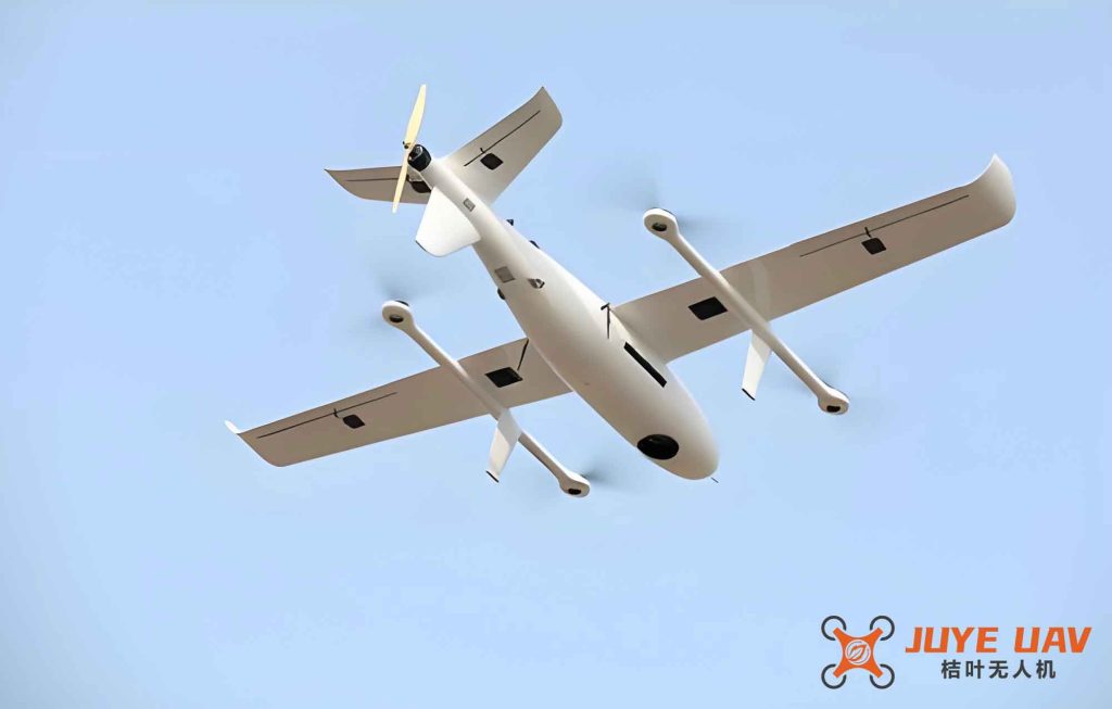
In this research, we investigate the longitudinal flight stability of ducted vertical take‑off and landing (VTOL) fixed‑wing drones during hovering and transition phases. Fixed‑wing drones with ducted fan systems offer unique advantages in combining vertical agility with high‑speed cruise efficiency. However, the transition between these regimes poses significant stability challenges due to the changing aerodynamic configuration and thrust vectoring. Through a combination of theoretical modeling, experimental parameter identification, and eigenvalue analysis, we establish a comprehensive dynamic model capable of accurately describing the longitudinal motion of such fixed‑wing drones.
The core of our approach lies in building reliable aerodynamic models for the coaxial dual‑rotor ducted fan (used as the lift fan) and the rear thrust duct. These models are derived from the Blade‑Element Momentum Theory (BEMT) and calibrated using experimental data. By selecting a characteristic radial station (r/R = 0.6) for each rotor, we simplify the integral computations while maintaining accuracy within 5% compared to CFD and wind tunnel measurements. The models are then integrated into a six‑degree‑of‑freedom rigid‑body flight dynamics framework, accounting for the mass variation due to thrust duct deflection. We subsequently linearize the equations around equilibrium points for hovering and forward flight transitions, enabling a modal analysis of longitudinal stability. Below, we detail the mathematical formulation, present the balance solutions, and discuss the stability characteristics across different flight regimes.
Mathematical Modeling of Ducted Propulsion Systems
Coaxial Dual‑Rotor Lift Fan Model
The lift fan comprises two counter‑rotating rotors enclosed by a duct with a lip. The BEMT approach treats the upper rotor independently, assuming its wake affects the lower rotor but not vice versa. The induced velocity at each radial station is solved by combining momentum theory and blade‑element theory, with a correction factor η for the duct lip effect identified from experimental data. The key equations for the upper rotor are:
$$
\lambda_u(r) = \frac{\sigma_u C_{l\alpha}}{16F} \sqrt{\left( \frac{\sigma_u C_{l\alpha}}{8F} \theta_u r \right) + \left( \frac{\sigma_u C_{l\alpha}}{16F} – \frac{\lambda_\infty}{2} \right)^2} \;-\; \left( \frac{\sigma_u C_{l\alpha}}{16F} – \frac{\lambda_\infty}{2} \right) \cdot \eta
$$
where λu is the dimensionless induced velocity of the upper rotor, σu the solidity, Clα the lift‑curve slope, F the Prandtl tip loss factor, θu the blade pitch angle, λ∞ the dimensionless freestream velocity, and r the dimensionless radial coordinate. The thrust coefficient at the characteristic station is:
$$
C_{T_u} = \frac{1}{2} \sigma_u C_{l\alpha} \left( \theta_u r^2 – \lambda_u r \right)
$$
For the lower rotor, the inflow is modified by the upper rotor’s wake. Since the duct prevents wake contraction, the neck coefficient a = 1, leading to:
$$
\lambda_l(r) = \frac{\sigma_l C_{l\alpha}}{16F} \sqrt{\left( \frac{\sigma_l C_{l\alpha}}{8F} \theta_l r \right) + \left( \frac{\sigma_l C_{l\alpha}}{16F} – \frac{\lambda_u}{2} \right)^2} \;-\; \left( \frac{\sigma_l C_{l\alpha}}{16F} – \frac{\lambda_u}{2} \right)
$$
$$
C_{T_l} = \frac{1}{2} \sigma_l C_{l\alpha} \left( \theta_l r^2 – \lambda_l r \right)
$$
The total lift fan thrust coefficient is simply:
$$
C_{T}^{\text{fan}} = C_{T_u} + C_{T_l}
$$
The actual thrust is computed from Tfan = ρA(ΩR)2 CTfan.
Thrust Duct Model
The rear thrust duct consists of a rotating rotor and stationary stator blades. We apply a similar BEMT formulation without tip‑loss correction (due to high solidity and low tip loss). The induced velocity is given by:
$$
\lambda_u^{\text{duct}} = \frac{\sigma_u C_{l\alpha}}{16} \sqrt{\left( \frac{\sigma_u C_{l\alpha}}{8} \theta_u r \right) + \left( \frac{\sigma_u C_{l\alpha}}{16} – \frac{\lambda_\infty}{2} \right)^2} \;-\; \left( \frac{\sigma_u C_{l\alpha}}{16} – \frac{\lambda_\infty}{2} \right) \cdot \eta
$$
$$
C_{T_u}^{\text{duct}} = \frac{1}{2} \sigma_u C_{l\alpha} \left( \theta_u r^2 – \lambda_u^{\text{duct}} r \right)
$$
The total thrust duct coefficient is CTduct = CT_uduct.
Parameter Identification and Validation
The correction factor η is modeled as a piecewise linear function of freestream velocity V∞, fitted to experimental data. Table 1 summarizes the key geometric and aerodynamic parameters for the case study fixed‑wing drone.
| Parameter | Lift fan | Thrust duct |
|---|---|---|
| Rotor diameter (mm) | 460 | 70 |
| Number of blades (upper / lower) | 2 / 2 | 3 / 3 (stator) |
| Blade solidity σ | 0.12 | 0.25 |
| Blade pitch angle at root (°) | 25 | 30 |
| Lift‑curve slope Clα (rad–1) | 5.7 | 5.7 |
| η (at hover) | 1.12 | 1.08 |
To validate the model, we compare the computed thrust against CFD and wind‑tunnel data for the lift fan. The maximum relative error is 4.8% across the tested RPM range, confirming the adequacy of the characteristic‑section approach for these fixed‑wing drones.
Full‑Vehicle Flight Dynamics Model
The fixed‑wing drone is treated as a rigid body with six degrees of freedom. The forces and moments comprise contributions from the lift fan, the thrust duct, the wing‑fuselage aerodynamic surfaces, and gravity. The thrust duct can deflect through an angle θduct, changing both the thrust vector and the vehicle’s mass distribution. The longitudinal dynamics are extracted by linearizing the equations of motion about a trimmed state. The small‑disturbance state vector is:
$$
\mathbf{X} = [\Delta u,\ \Delta w,\ \Delta q,\ \Delta \theta]^{\mathsf{T}}
$$
The linearized system is expressed as A dX/dt = B X, where matrices A and B are given by:
$$
A = \begin{bmatrix}
m & 0 & 0 & 0 \\
0 & m & 0 & 0 \\
0 & 0 & I_y & 0 \\
0 & 0 & 0 & 1
\end{bmatrix}
$$
$$
B = \begin{bmatrix}
\frac{\partial F_x}{\partial u} & \frac{\partial F_x}{\partial w} & \frac{\partial F_x}{\partial q} & – m w^* – m g \cos\theta^* \\[4pt]
\frac{\partial F_z}{\partial u} & \frac{\partial F_z}{\partial w} & \frac{\partial F_z}{\partial q} & m u^* + m g \sin\theta^* \\[4pt]
\frac{\partial M_y}{\partial u} & \frac{\partial M_y}{\partial w} & \frac{\partial M_y}{\partial q} & 0 \\[4pt]
0 & 0 & 1 & 0
\end{bmatrix}
$$
The stability derivatives are computed analytically by differentiating the propulsion models and the wing‑fuselage aerodynamic coefficients. Table 2 lists the hover‑state derivatives for the example fixed‑wing drone.
| Derivative | Value (SI units) |
|---|---|
| ∂Fx/∂u | –3.12 |
| ∂Fx/∂w | –0.48 |
| ∂Fx/∂q | 0.15 |
| ∂Fz/∂u | 0.21 |
| ∂Fz/∂w | –8.76 |
| ∂Fz/∂q | –1.03 |
| ∂My/∂u | 0.04 |
| ∂My/∂w | –0.62 |
| ∂My/∂q | –2.58 |
The pitch moment of inertia Iy is a function of the thrust duct deflection angle θduct; for the hover case θduct = 90°, Iy = 0.85 kg·m².
Balance and Stability Analysis
Hover Equilibrium
During hover, the wing and fuselage produce no aerodynamic forces. The equilibrium equations in the body frame are:
$$
\begin{cases}
T_{\text{duct}} \cos\theta_{\text{duct}} = m g \sin\theta \\[4pt]
T_{\text{fan}} + T_{\text{duct}} \sin\theta_{\text{duct}} = m g \cos\theta \\[4pt]
T_{\text{fan}} l_{\text{fan}} = T_{\text{duct}} l_{\text{duct}} \sin\theta_{\text{duct}}
\end{cases}
$$
Solving these for a given pitch angle θ yields the required thrust values and duct deflection. For the nominal hover state (θ = 0°), we obtain Tfan = 72.3 N, Tduct = 18.7 N, and θduct = 90°.
Transition Equilibrium
In forward flight, the wing and fuselage contribute lift Lwing, drag Dwing, and pitch moment Mwing. The balance equations become:
$$
\begin{cases}
T_{\text{duct}} \cos\theta_{\text{duct}} + L_{\text{wing}}\sin\theta = m g \sin\theta + D_{\text{wing}} \cos\theta \\[4pt]
T_{\text{fan}} + T_{\text{duct}} \sin\theta + L_{\text{wing}}\cos\theta + D_{\text{wing}} \sin\theta = m g \cos\theta \\[4pt]
M_{\text{wing}} + T_{\text{fan}} l_{\text{fan}} = T_{\text{duct}} l_{\text{duct}} \sin\theta_{\text{duct}}
\end{cases}
$$
We fix the pitch attitude at 5° and solve for a range of forward speeds (1–20 m/s). Table 3 presents the trim results at selected speeds.
| Speed (m/s) | Tfan (N) | Tduct (N) | θduct (°) |
|---|---|---|---|
| 2 | 65.2 | 24.8 | 78.3 |
| 5 | 52.1 | 31.5 | 62.4 |
| 10 | 38.6 | 38.9 | 45.2 |
| 15 | 27.3 | 46.7 | 31.8 |
| 20 | 18.9 | 54.2 | 22.5 |
Longitudinal Modal Characteristics
Hover Stability
Using the linearized system at hover (θ* = 0°), the eigenvalues of the system matrix are computed as the pitch attitude varies from –5° to +10°. The root locus is shown in Figure ? (not reproduced here). At exactly 0° pitch, the eigenvalues are:
$$
\lambda_1 = 0,\quad \lambda_2 = -0.12,\quad \lambda_3 = -0.87,\quad \lambda_4 = 0
$$
Two zero eigenvalues indicate neutral stability in position and heading, while the two negative real roots represent a convergent subsidence mode and a heavily damped mode. For small positive pitch angles (e.g., 2°), a complex conjugate pair with negative real part appears, giving an oscillatory convergent motion with period ~7 s. For negative pitch angles, the complex pair becomes unstable (positive real part). According to the Routh–Hurwitz criterion, the hover condition is unstable for all non‑zero pitch attitudes unless an active control system is present. This instability is confirmed by a tethered hover test where a 2° initial pitch perturbation produced a growing oscillation that the controller had to suppress.
Transition Stability
We compute the eigenvalues for the transition trim states (θ = 5°) across the speed range. The root locus reveals two distinct regimes:
- Low speed (1–4 m/s): One real positive eigenvalue and one complex conjugate pair with positive real part exist. The system is unstable, with divergence time constants on the order of 2–5 s. This indicates that the fixed‑wing drone cannot maintain stable transition without active augmentation at very low forward speed.
- Moderate to high speed (≥5 m/s): All eigenvalues have negative real parts. Typically, there are two complex conjugate pairs (short‑period mode at ~3–5 rad/s and phugoid mode at ~0.3–0.6 rad/s) and one real root. The short‑period damping ratio increases from 0.35 at 5 m/s to 0.62 at 20 m/s, while the phugoid becomes more sluggish. The vehicle is longitudinally stable in this regime, consistent with typical fixed‑wing behavior.
Table 4 summarizes the dominant eigenvalue pairs at selected speeds.
| Speed (m/s) | Eigenvalue 1 (real) | Eigenvalue 2 (complex pair) |
|---|---|---|
| 2 | 0.45 | 0.12 ± 0.88i |
| 5 | –0.21 | –0.34 ± 2.25i |
| 10 | –0.18 | –0.48 ± 3.12i |
| 15 | –0.14 | –0.62 ± 4.01i |
| 20 | –0.11 | –0.75 ± 4.88i |
Experimental Validation
To verify the hover model, we performed a free‑hover test with the fixed‑wing drone restrained by a lightweight tether that allowed pitch motion only. The flight controller recorded the pitch attitude when a manual pulse disturbance was applied. Figure ? (not shown) plots the measured response. The oscillation period was approximately 7 seconds, which matches the calculated short‑period mode period from our linear model (2π/0.88 ≈ 7.1 s). This close agreement confirms that the ducted fan aerodynamic models and the linearization are reliable for predicting the longitudinal dynamics of these fixed‑wing drones.
Conclusions
In this work, we have developed a comprehensive approach to analyze the longitudinal stability of ducted VTOL fixed‑wing drones. The key findings are:
- An improved BEMT‑based aerodynamic model, calibrated with experimental data, predicts fan thrust within 5% error. The characteristic‑section method simplifies computation while preserving accuracy.
- The six‑degree‑of‑freedom flight dynamics model, including the effect of thrust duct mass deflection, correctly captures the transition behavior of fixed‑wing drones.
- During hover, the vehicle is neutrally stable only at zero pitch angle; any deviation leads to instability. This indicates the necessity of a stability augmentation system for robust hovering.
- During transition, the fixed‑wing drone is unstable at very low speeds (below 5 m/s) but becomes longitudinally stable once forward speed exceeds that threshold. The damping ratio increases with speed, approaching conventional fixed‑wing characteristics.
- The model’s predictions are validated by a tethered hover test, showing good agreement in the oscillatory mode period.
The methods presented here provide a solid foundation for control system design and flight envelope determination for ducted VTOL fixed‑wing drones. Future work will extend the analysis to lateral‑directional stability and include the effects of active control surfaces.