
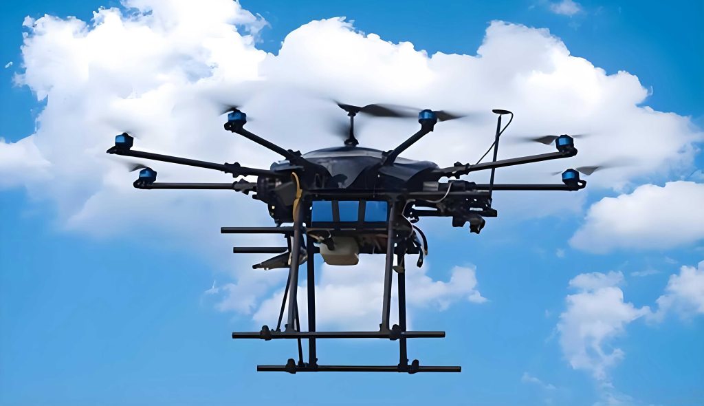
The precise measurement and assessment of forest structure is paramount for sustainable forest management and ecological studies. Key structural parameters of individual trees, such as diameter at breast height (DBH), height, crown diameter, and volume, are fundamental for analyzing forest function, biomass estimation, and conservation planning. Light Detection and Ranging (LiDAR) technology has revolutionized forest inventory by enabling the direct, efficient, and three-dimensional acquisition of structural information. Among the various platforms, Unmanned Aerial Vehicle (UAV) mounted LiDAR systems, or UAV drones, have emerged as a particularly powerful tool. They offer a unique balance between the extensive coverage of traditional airborne laser scanning (ALS) and the high detail of terrestrial laser scanning (TLS), often at a lower operational cost and with greater flexibility.
Most existing methods for individual tree detection (ITD) from UAV drone point clouds inherit strategies developed for ALS data, predominantly following a top-down paradigm. These methods focus on delineating tree crowns based on features derived from the canopy surface, utilizing algorithms like region growing, watershed segmentation, or clustering on canopy height models (CHMs) or the point cloud itself. While effective in open or uniformly structured forests, their performance often degrades in complex, multi-layered stands with dense, overlapping crowns because they rely heavily on the often ambiguous and irregular geometry of the crown surface. Conversely, methods developed for TLS data leverage the detailed understory information, following a bottom-up paradigm by first detecting tree stems and then assigning crown points. However, these methods are critically dependent on accurate stem detection, which can be challenging from a top-down UAV drone perspective due to occlusion by foliage.
This highlights a significant gap: the unique data characteristics of UAV drone LiDAR, which simultaneously capture reasonable crown detail and partial stem information (especially for dominant and co-dominant trees), are not fully exploited. The stem points, though sparser than in TLS, provide valuable vertical structural anchors that are largely ignored by top-down methods. Therefore, I propose a novel methodology that synergistically fuses information from both tree crowns and stems extracted from UAV drone point clouds to achieve more robust and accurate individual tree delineation in varied forest conditions.
Methodology
The proposed framework is designed to intelligently combine the horizontal extent information from tree crowns with the vertical positional certainty from tree stems. The core philosophy is to use an initial crown segmentation as a basis, identify its potential flaws (over-segmentation and under-segmentation) using stem-derived cues, and then apply a refined graph-cut segmentation that is guided by both crown shape and stem location. The complete workflow is illustrated below and detailed in the subsequent sections.
1. Data Preprocessing and Initial Crown Segmentation
The raw point cloud from the UAV drone is first processed to isolate vegetation points. Ground points are filtered out using an algorithm such as Cloth Simulation Filter (CSF). Subsequently, low vegetation (e.g., shrubs) is removed by applying a height threshold relative to the digital terrain model (DTM), typically around 2 meters. The remaining points are considered potential tree points.
An initial segmentation of tree crowns is performed using the Mean Shift clustering algorithm with an asymmetric kernel. This method is effective for segmenting the dense, mound-like structures of tree crowns in a top-down view. It operates directly on the 3D points, iteratively shifting points towards the mode (highest density) of their local neighborhood. The bandwidth parameters control the scale of the segments. This step partitions the forest area into a set of initial clusters, each ideally corresponding to one tree crown. However, in reality, these initial clusters often contain errors: a single cluster may encompass multiple overlapping trees (under-segmentation), or a single tree crown may be split into several clusters (over-segmentation).
2. Stem Detection and Characterization
Concurrently, a dedicated process detects tree stems. This is a critical step that leverages the vertical structure captured by UAV drones. I employ a point-wise classification approach based on Random Forest. For each point below a certain height (e.g., within 1-5 meters above ground), a set of geometric features is calculated within its local neighborhood (e.g., a sphere of 0.2m radius). These features are designed to distinguish the linear, cylindrical structure of tree stems from the planar (leaves) or scattered (branches, shrubs) points.
The feature set includes standard eigenvalue-based features derived from the covariance matrix of the local neighborhood, as well as specifically designed “Significance of Difference” features to enhance separability. For a point with linearity $(L)$, planarity $(P)$, and sphericity $(S)$ features (where $L+P+S=1$), the Significance of Difference for Planarity ($SoDP$) and Sphericity ($SoDS$) are defined as:
$$
SoDP = P + (1 – P) \times [P – \max(L, S)]
$$
$$
SoDS = S + (1 – S) \times [S – \max(L, P)]
$$
These features amplify the characteristic geometric trait of a point relative to the others. A stem point typically has high $L$ and high $SoDP$ (as it is more planar than scattered in a cross-section). A comprehensive list of features used for stem classification is summarized in Table 1.
| Feature | Description |
|---|---|
| $\lambda_1, \lambda_2, \lambda_3$ | Eigenvalues ($\lambda_1 \geq \lambda_2 \geq \lambda_3 \geq 0$) |
| Linearity ($L$) | $(\lambda_1 – \lambda_2) / \lambda_1$ |
| Planarity ($P$) | $(\lambda_2 – \lambda_3) / \lambda_1$ |
| Sphericity ($S$) | $\lambda_3 / \lambda_1$ |
| Omnivariance | $\sqrt[3]{\lambda_1 \lambda_2 \lambda_3}$ |
| Anisotropy | $(\lambda_1 – \lambda_3) / \lambda_1$ |
| Eigenentropy | $- \sum_{i=1}^{3} \lambda_i \ln(\lambda_i)$ |
| Sum of $\lambda$ | $\lambda_1 + \lambda_2 + \lambda_3$ |
| Curvature | $\lambda_3 / (\lambda_1 + \lambda_2 + \lambda_3)$ |
| $SoDP$ | Significance of Difference for Planarity (Eq. 1) |
| $SoDS$ | Significance of Difference for Sphericity (Eq. 2) |
| FPFH (simplified) | Fast Point Feature Histogram (angular relationships) |
A Random Forest classifier is trained on a small manually labeled dataset to distinguish “Stem” from “Non-Stem” points. The classified stem points are then clustered in 2D (X-Y plane) using a 2D Mean Shift algorithm to group points belonging to the same physical stem. Finally, these stem clusters are refined (e.g., by removing clusters with too few points or unrealistic dimensions) to produce the final set of detected tree stems, each represented by its 2D location $(x, y)$ and an approximate height.
3. Identification of Over- and Under-Segmented Crown Clusters
The initial crown clusters from Step 1 are now analyzed in conjunction with the detected stems from Step 2. The key idea is that a correctly segmented single tree crown should be associated with, at most, one stem directly beneath it. Conversely, an under-segmented cluster (containing multiple trees) will likely have multiple stems within its projected area, while an over-segmented cluster (part of a single crown) may have no stem or its associated stem may conflict with another cluster’s stem.
I construct a set of features for each initial crown cluster that describe its morphology and its relationship with stems. These features are used to train another Random Forest model to classify each cluster as “Correct,” “Over-segmented,” or “Under-segmented.” The feature set is summarized in Table 2.
| Category | Feature | Description |
|---|---|---|
| Crown Morphology | $D_{min}$, $D_{max}$ | Min and max diameter of the cluster’s 2D convex hull. |
| $C_d$ | Mean crown diameter: $(D_{min} + D_{max}) / 2$. | |
| $R_d$ | Aspect ratio: $D_{min} / D_{max}$. | |
| $Area_{proj}$ | Area of the 2D convex hull of the cluster. | |
| $Height$ | $Z_{max} – Z_{min}$ of the cluster. | |
| $Z_{max}$ | Maximum Z (height) of the cluster. | |
| Allometric Check | $C_e$ | Expected crown diameter from allometry: $C_e = \alpha \cdot Height^{\beta}$ (e.g., 0.446·$Height^{0.854}$). |
| $R_C$ | Relative crown size difference: $(C_d – C_e) / C_e$. | |
| – | – | |
| Stem Relation | $N_s$ | Number of detected stems within the cluster’s 2D projected polygon. |
| $Dist_{stem}$ | Distance from cluster centroid to the nearest stem. | |
| Cluster Property | $Variance_{MS}$ | Variance of points around the mode found by Mean Shift. |
Based on the classification, over-segmented clusters adjacent to an under-segmented one are merged with it. A simple allometric constraint prevents merging unrelated segments: if the distance between an over-segmented part and the candidate under-segmented cluster exceeds half of the expected crown width ($C_e/2$) of the over-segmented part, the merge is rejected, and the over-segmented part is promoted to a potential single tree.
4. Refined Segmentation via Tree-Centric Vector-Angle Optimized Graph Cut
The clusters identified as “Under-segmented” and the merged clusters require precise boundary delineation to separate individual trees. For this, I employ a graph-cut segmentation method that is specifically optimized using both crown and stem information. Graph-cut formulates segmentation as an energy minimization problem on a graph, where each point is a node.
For an under-segmented cluster containing $N$ stems, the process is run $N$ times to extract each tree. For the $k$-th stem, the graph is constructed as follows:
- Source (Foreground): The points belonging to the target stem $k$.
- Sink (Background): A collective set of points from all other stems ($\neq k$) within the cluster and any other “background” stems from nearby trees.
- Other Points: All non-stem vegetation points within the bounding region of the under-segmented cluster.
The goal is to label each “other point” as either belonging to the target tree (connected to source) or not (connected to sink). The energy function has two main costs:
- Data Cost (Penalty): Assigns a cost for assigning a point to the source or sink.
- Foreground Penalty ($w_f$): A constant low cost for connecting to the source.
- Background Penalty ($w_b$): A cost based on the 2D horizontal distance from the point to the target stem ($dist_{2d}$) and the expected crown radius ($R_{est}$) derived from the stem’s height: $$ w_{b\_dist} = \frac{dist_{2d}}{R_{est}} $$
- Smoothness Cost: Penalizes differences in labeling between neighboring points $i$ and $j$. It is defined to encourage cuts where there is a significant 3D gap: $$ smoothCost(i,j) = \exp\left(-\frac{||(x,y)_i – (x,y)_j||^2}{\sigma_{xy}^2} – \frac{(z_i – z_j)^2}{\sigma_{z}^2}\right) $$ where $\sigma_{xy}$ and $\sigma_{z}$ control the sensitivity in horizontal and vertical dimensions.
The key innovation is the enhancement of the background penalty using tree-centric directional information. For each point $i$ in the cluster, I estimate its direction vector pointing towards the center of the crown mass it likely belongs to. This is done by performing a local 2D adaptive mean-shift procedure on the horizontal coordinates of points within a local vertical column around $i$. The resulting shift vector $\vec{D}_{crown}(i)$ points towards the local crown center. Simultaneously, I define the vector from point $i$ to the target stem $k$ as $\vec{D}_{stem}(i, k)$.
The deviation angle $\theta_i$ between these two vectors indicates how well the point’s local crown structure aligns with the target stem:
$$
\theta_i = \arccos\left(\frac{\vec{D}_{crown}(i) \cdot \vec{D}_{stem}(i, k)}{||\vec{D}_{crown}(i)|| \cdot ||\vec{D}_{stem}(i, k)||}\right)
$$
A small $\theta_i$ suggests the point’s crown mass is centered around the target stem, making it more likely to belong to that tree. This angular information is converted into an angular penalty weight $w_\theta$:
$$
w_\theta(i) = -\gamma \cdot \exp\left(-\frac{\pi – \theta_i}{\phi}\right)
$$
where $\gamma$ and $\phi$ are parameters controlling the strength and sensitivity of the angular term. A negative sign is used so that a small angle (good alignment) results in a lower (more negative) total background cost, encouraging the point to be assigned to the foreground.
The final background penalty for the graph-cut is a weighted combination of the distance-based and angle-based penalties:
$$
w_{b\_final}(i) = \omega \cdot w_{b\_dist}(i) + (1 – \omega) \cdot w_{\theta}(i)
$$
where $\omega$ is a blending parameter. This composite penalty allows the graph-cut to find boundaries that are not only spatially compact but also consistent with the internal crown geometry relative to the stem position. The minimized cut then yields the final set of points belonging to the individual tree associated with stem $k$.
Experimental Analysis and Results
The proposed method was evaluated on four distinct UAV drone LiDAR datasets acquired from various forest types and geographical locations to assess its robustness. The characteristics of 15 sample plots extracted from these datasets are summarized in Table 3, covering mixed, coniferous, and broadleaf forests with a range of tree heights and densities.
| Dataset | Plot ID | Forest Type | Avg. Tree Height (m) | Stem Density (trees/ha) |
|---|---|---|---|---|
| I (Germany) | 1 | Mixed Conifer-Broadleaf | 28 | 304 |
| 2 | Mixed Conifer-Broadleaf | 39 | 368 | |
| 3 | Mixed Conifer-Broadleaf | 43 | 272 | |
| 4 | Mixed Conifer-Broadleaf | 28 | 224 | |
| II (Netherlands) | 5 | Coniferous | 31 | 231 |
| 6 | Coniferous | 20 | 714 | |
| III (China) | 7 | Broadleaf (Plantation) | 22 | 122 |
| 8 | Broadleaf (Plantation) | 20 | 100 | |
| 9 | Broadleaf (Plantation) | 19 | 133 | |
| 10 | Broadleaf (Plantation) | 21 | 100 | |
| IV (Multi-country) | 11 | Coniferous | 29 | 612 |
| 12 | Coniferous | 32 | 959 | |
| 13 | Coniferous | 30 | 650 | |
| 14 | Coniferous | 33 | 390 | |
| 15 | Coniferous | 30 | 244 |
Reference data (individual tree polygons) were manually delineated for each plot. Performance was evaluated using standard metrics:
- Precision: $TP / (TP + FP)$
- Recall: $TP / (TP + FN)$
- F1-Score: $2 \times (Precision \times Recall) / (Precision + Recall)$
- Mean Intersection over Union (mIOU): $\frac{1}{N} \sum \frac{|T_{pred} \cap T_{ref}|}{|T_{pred} \cup T_{ref}|}$, where a match is validated if $IOU > 0.5$.
Here, $TP$ (True Positive) is a correctly detected tree, $FP$ (False Positive) is a detected tree with no real match, and $FN$ (False Negative) is a real tree not detected.
Overall Delineation Performance
The quantitative results across all 15 plots are presented in Table 4. The method achieved an average mIOU of 87.2%, indicating high spatial congruence between the extracted and reference tree segments. The average Precision, Recall, and F1-Score were all 0.82, demonstrating a balanced and accurate detection capability across diverse forest structures captured by the UAV drones.
| Plot ID | mIOU | Precision | Recall | F1-Score |
|---|---|---|---|---|
| 1 | 84.1% | 0.70 | 0.75 | 0.72 |
| 2 | 90.7% | 0.91 | 1.00 | 0.95 |
| 3 | 83.8% | 0.70 | 0.70 | 0.70 |
| 4 | 90.2% | 0.61 | 0.69 | 0.65 |
| 5 | 87.9% | 0.96 | 0.92 | 0.94 |
| 6 | 79.9% | 0.81 | 0.66 | 0.73 |
| 7 | 86.7% | 1.00 | 1.00 | 1.00 |
| 8 | 90.0% | 0.92 | 0.85 | 0.88 |
| 9 | 93.4% | 1.00 | 0.91 | 0.95 |
| 10 | 88.0% | 0.90 | 0.90 | 0.90 |
| 11 | 94.7% | 0.94 | 0.94 | 0.94 |
| 12 | 88.8% | 0.86 | 0.81 | 0.84 |
| 13 | 90.5% | 0.71 | 0.61 | 0.66 |
| 14 | 77.2% | 0.63 | 0.60 | 0.62 |
| 15 | 82.0% | 0.69 | 0.96 | 0.80 |
| Average | 87.2% | 0.82 | 0.82 | 0.82 |
Ablation Study: Efficacy of the Tree-Centric Vector-Angle Optimization
To validate the contribution of the novel tree-centric vector-angle penalty, I compared the final segmentation results against those obtained using a standard graph-cut with only the distance-based penalty ($w_{b\_dist}$). The comparison, shown in Table 5, focuses on the plots where the refinement step was actively used (primarily plots with under-segmentation). The proposed optimization consistently improved or maintained the F1-Score and mIOU. The standard graph-cut often produced overly compact segments or failed to correctly assign points in complex crown overlaps, whereas the angle-guided penalty better captured the natural crown expansion from the stem, leading to more accurate boundaries.
| Plot ID | Proposed Method (Angle-Optimized) | Standard Graph-Cut (Distance Only) | ||
|---|---|---|---|---|
| mIOU | F1-Score | mIOU | F1-Score | |
| 1 | 84.1% | 0.72 | 84.1% | 0.71 |
| 2 | 90.7% | 0.95 | 90.6% | 0.91 |
| 3 | 83.8% | 0.70 | 81.2% | 0.58 |
| 4 | 90.2% | 0.65 | 94.5% | 0.63 |
| 11 | 94.7% | 0.94 | 95.2% | 0.92 |
| 12 | 88.8% | 0.84 | 82.0% | 0.84 |
| 13 | 90.5% | 0.66 | 85.9% | 0.67 |
| 14 | 77.2% | 0.62 | 72.6% | 0.49 |
| 15 | 82.0% | 0.80 | 82.6% | 0.73 |
Comparative Analysis with State-of-the-Art Methods
I compared the overall performance of the proposed method against three representative approaches from the literature, as shown in Table 6:
- Bottom-up Graph-Cut (TLS-style): A method that first detects stems and uses a simple graph-cut for crown delineation. Its low performance (Precision=0.29, Recall=0.21) on UAV drone data underscores the challenge of reliable stem detection from a nadir view and the insufficiency of basic graph-cut without crown-stem fusion.
- Top-down Region Growing (ALS/ULS-style): A method that grows crowns from local maxima on a CHM. Its moderate results (F1=0.62) suffer in dense stands due to crown overlap and the lack of vertical structural information.
- CHM-based Local Maxima Clustering: A common ITD method using a smoothed CHM. It performed reasonably well (F1=0.73) but was outperformed by the proposed method, particularly in recall, as it misses trees hidden in the canopy layer.
| Method | Paradigm | Avg. mIOU | Avg. Precision | Avg. Recall | Avg. F1-Score |
|---|---|---|---|---|---|
| Proposed Method | Crown-Stem Fusion | 87.2% | 0.82 | 0.82 | 0.82 |
| Bottom-up Graph-Cut | Stem-based (TLS-style) | 50.4% | 0.29 | 0.21 | 0.23 |
| Top-down Region Growing | Crown-based (ALS-style) | 81.3% | 0.62 | 0.68 | 0.62 |
| CHM Local Maxima Clustering | Crown-based (CHM) | 84.5% | 0.76 | 0.70 | 0.73 |
The proposed method’s superior performance stems from its hybrid strategy. It mitigates the limitations of pure top-down methods by using stems to validate and correct crown segments. It also overcomes the stem-detection dependency of pure bottom-up methods by using the initial crown segmentation as a guide and a fallback. The tree-centric vector-angle optimization is the crucial link that allows these two information streams to interact effectively during the precise boundary delineation phase.
Conclusion
This work presents a robust framework for individual tree delineation from UAV drone LiDAR point clouds by fusing complementary information from tree crowns and stems. The methodology moves beyond the traditional top-down/bottom-up dichotomy by establishing a synergistic relationship between the two structural components. The initial crown segmentation provides a scalable region-of-interest, while stem detection offers unambiguous positional anchors. The intelligent classification of segmentation errors and the subsequent refined graph-cut segmentation, optimized with a novel tree-centric vector-angle penalty, effectively handle complex crown overlaps and deliver accurate tree boundaries.
The experimental results across diverse forest environments demonstrate that the method achieves a balanced and high performance (mIOU=87.2%, F1=0.82), outperforming conventional approaches that rely solely on crown or stem information. This confirms the significant value of leveraging the full 3D structural information inherent in modern UAV drone LiDAR data.
Future work will focus on enhancing stem detection robustness in extremely dense understories and refining the allometric and geometric models used for cluster analysis. Furthermore, exploring the integration of multispectral or hyperspectral data from UAV drones could allow for simultaneous species classification and structural delineation, paving the way for comprehensive and automated forest analytics using versatile UAV drone platforms.