
In my research, I focus on the challenging problem of three-dimensional path planning for UAV drones in complex low-altitude environments. The rapid growth of low-altitude economies, advanced communication infrastructure, and intelligent control technologies has made UAV drones increasingly common in tasks such as search and patrol, reconnaissance, emergency rescue, logistics delivery, power inspection, agricultural meteorology, and urban security. Because UAV drones can adapt flexibly to complex and changing environments and respond quickly to emergencies without risking human life, their operational scope continues to expand. However, the core of safe and efficient UAV drone operation lies in path planning. A well-designed path planning algorithm must generate a feasible, low-cost, and safe trajectory from a starting point to a destination while satisfying multiple constraints, including flight altitude, turning angle, climb and dive angle, path length, and obstacle avoidance. In my work, I systematically improve two swarm intelligence optimization algorithms to address the distinct characteristics of mountainous terrain and dense urban areas. The proposed methods are validated through benchmark functions, simulation environments, and real-world flight tests on a custom UAV drone platform.
UAV drones are now widely deployed in fields such as disaster relief, power line inspection, light shows, and agricultural plant protection. Their ability to operate in hazardous or inaccessible areas makes them indispensable tools for modern society. Nevertheless, path planning for UAV drones remains a difficult optimization problem because the search space is high-dimensional, non-convex, and subject to multiple physical constraints. In mountainous regions, terrain undulations are severe, peaks are dense, and elevation surfaces change continuously. In urban regions, buildings are densely packed, regular obstacles are abundant, and available flight corridors are narrow. These two types of environments demand different algorithmic capabilities. For mountainous terrain, the planner must handle continuous elevation surfaces and frequent climb and dive maneuvers. For urban terrain, the planner must avoid dense rule-based obstacles and find feasible paths through limited free space. My research therefore develops two tailored algorithms: a multi-strategy improved hippopotamus optimization algorithm for mountainous UAV drone path planning, and a multi-strategy improved honey badger algorithm for urban UAV drone path planning.
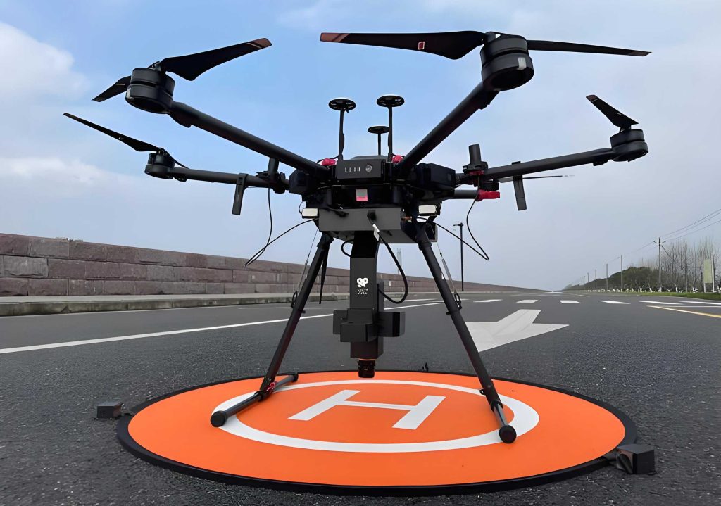
Swarm intelligence optimization algorithms simulate the social behaviors of biological populations to find optimal or near-optimal solutions at low computational cost. They are simple, easy to implement, and widely used in path planning. However, traditional swarm intelligence algorithms often suffer from weak randomness, slow convergence, low accuracy, the curse of dimensionality in three-dimensional space, and poor adaptability to different terrain features. Therefore, targeted improvements are necessary. In my study, I use improved hippopotamus optimization for mountainous UAV drone path planning to handle continuous elevation surfaces. For urban UAV drone path planning, I improve the honey badger algorithm to enhance feasibility in dense obstacle environments.
Related Principles and Problem Formulation
Before presenting my proposed algorithms, I introduce the fundamental principles of three-dimensional environment modeling, path planning objective functions, algorithm evaluation, and path smoothing. These principles form the basis for the experimental design and performance analysis.
Three-Dimensional Environment Modeling
Traditional two-dimensional environment modeling cannot satisfy path planning tasks in mountainous rescue, mountain breakout, or urban logistics where altitude changes are critical. Therefore, a three-dimensional environment map is essential. The flight region of a UAV drone is bounded as follows:
$$0 \leq x \leq x_{\max}, \quad 0 \leq y \leq y_{\max}, \quad 0 \leq z \leq z_{\max}$$
Two common modeling methods are the three-dimensional grid map and the digital elevation model. The grid map discretizes the planning space into identical cubic cells, each storing occupancy information. The digital elevation model uses ordered numerical arrays to represent ground elevation, producing a continuous and smooth elevation surface. I adopt the regular grid form of the digital elevation model because it has a simple data structure, clear topological relationships, and high computational efficiency. The elevation value of each grid can be obtained by a mathematical model:
$$z = f(x,y)$$
where \(z\) represents the environmental elevation corresponding to the horizontal coordinate \((x,y)\). This continuous function allows me to construct realistic mountainous terrain with peaks, slopes, and valleys.
Path Planning Objective Function and Constraints
The minimum flight height \(H_{\min}\) is the minimum height above ground that a UAV drone must maintain. For any flight segment \(i\), the constraint is:
$$H_i \geq H_{\min}, \quad i = 1,2,\ldots,n$$
The minimum path segment length \(l_{\min}\) is the shortest straight-line distance that a UAV drone must maintain before changing its flight attitude. If a path consists of \(n\) segments \(l_i\), each segment must satisfy:
$$l_i \geq l_{\min}$$
The maximum turning angle \(\phi\) restricts the horizontal turn of a UAV drone. Let the horizontal projection of segment \(i\) be:
$$\mathbf{a}_i = [x_i – x_{i-1}, \; y_i – y_{i-1}]^T$$
Then the maximum turning angle constraint is:
$$\frac{\mathbf{a}_i^T \mathbf{a}_{i+1}}{\|\mathbf{a}_i\| \cdot \|\mathbf{a}_{i+1}\|} \geq \cos\phi, \quad i = 2,3,\ldots,n-1$$
The maximum climb angle and maximum dive angle \(\theta\) constrain vertical maneuvers. The constraint is:
$$\left|\frac{z_i – z_{i-1}}{\|\mathbf{a}_i\|}\right| \leq \tan\theta, \quad i = 2,3,\ldots,n$$
The maximum path length \(L_{\max}\) limits the total flight distance. The constraint is:
$$\sum_{i=1}^{n} l_i \leq L_{\max}$$
In my formulation, the path cost function \(C\) combines path length, height, and threat index:
$$C = \sum_{i=1}^{n} \left( \omega_1 l_i + \omega_2 h_i + \omega_3 g_i \right)$$
where \(h_i\) is the height above ground, \(g_i\) is the threat index, and \(\omega_1, \omega_2, \omega_3\) are weights satisfying \(\omega_1 + \omega_2 + \omega_3 = 1\). The path length is computed as the sum of Euclidean distances between adjacent nodes:
$$fit = \sum_{i=1}^{m} \sqrt{(x_{i+1} – x_i)^2 + (y_{i+1} – y_i)^2}$$
where \((x_i, y_i)\) and \((x_{i+1}, y_{i+1})\) are adjacent nodes and \(m\) is the total number of nodes.
Algorithm Evaluation Criteria
I evaluate my improved algorithms on the CEC2005 benchmark suite. This suite contains 23 functions divided into unimodal, multimodal, and fixed-dimension hybrid functions. Table 1 summarizes the categories and characteristics.
| Category | Functions | Characteristics |
|---|---|---|
| Unimodal | \(f_1\)–\(f_5\) | Single global optimum, simple structure, high-dimensional |
| Step and noisy | \(f_6\)–\(f_7\) | Discontinuous or noisy, tests robustness |
| Multimodal | \(f_8\)–\(f_{13}\) | Many local optima, steep and narrow peaks |
| Fixed-dimension hybrid | \(f_{14}\)–\(f_{23}\) | Predefined dimensions, composite search spaces |
For performance evaluation, I use the mean and standard deviation over multiple independent runs. The mean is:
$$Mean = \frac{1}{S} \sum_{i=1}^{S} C_i$$
where \(S\) is the number of runs and \(C_i\) is the result of the \(i\)-th run. The standard deviation is:
$$Std = \sqrt{\frac{1}{S} \sum_{i=1}^{S} \left( C_i – \frac{1}{S} \sum_{j=1}^{S} C_j \right)^2}$$
I also use Friedman ranking and Wilcoxon signed-rank tests to compare algorithms statistically.
Cubic Spline Interpolation for Path Smoothing
To ensure flyability and smoothness, I apply cubic spline interpolation to the planned path. The spline is defined piecewise:
$$S_k(x) = a_k + b_k (x – x_k) + c_k (x – x_k)^2 + d_k (x – x_k)^3$$
where \(a_k, b_k, c_k, d_k\) are coefficients for the \(k\)-th subinterval, and \(x_k\) is the \(k\)-th node. The interpolation nodes are distributed as:
$$x_k = x_{\text{start}} + \frac{k}{m} (x_{\text{end}} – x_{\text{start}})$$
This smoothing step reduces oscillations and ensures that the UAV drone can follow the path without abrupt attitude changes.
Original Swarm Intelligence Algorithms
In this section, I briefly describe the two original algorithms that form the foundation of my improved methods: the hippopotamus optimization algorithm and the honey badger algorithm.
Hippopotamus Optimization Algorithm
The hippopotamus optimization algorithm simulates three typical behaviors of hippopotamus herds: position updating, defense, and escape. The population matrix is:
$$\mathbf{X} = \begin{bmatrix} x_{11} & \cdots & x_{1m} \\ \vdots & \ddots & \vdots \\ x_{N1} & \cdots & x_{Nm} \end{bmatrix}$$
where \(N\) is the population size and \(m\) is the dimension. The fitness matrix is:
$$\mathbf{F} = \begin{bmatrix} F(x_{11}, \ldots, x_{1m}) \\ \vdots \\ F(x_{N1}, \ldots, x_{Nm}) \end{bmatrix}$$
Initialization is performed as:
$$x_{ij} = lb_j + rand \cdot (ub_j – lb_j)$$
In the position updating phase, the male hippopotamus updates its position as:
$$X_i^{\text{Mhippo}}: x_{ij} = x_{ij} + y_1 \cdot (D_{\text{hippo}} – I_1 x_{ij})$$
Female and young hippos update as:
$$X_i^{\text{FBhippo}} = \begin{cases} x_{ij} + h_1 \cdot (D_{\text{hippo}} – I_2 MG), & T > 0.6 \\ x_{ij} + h_2 \cdot (MG – D_{\text{hippo}}), & \text{else} \end{cases}$$
The defense phase generates a predator position:
$$P_j = lb_j + r_6 \cdot (ub_j – lb_j)$$
The escape phase updates position as:
$$x_{ij}^{\text{Hs}} = x_{ij} + rand_3 \cdot (lb_j^{\text{local}} + s \cdot (ub_j^{\text{local}} – lb_j^{\text{local}}))$$
Lévy flight is also used in the defense phase:
$$Levy(w) = 0.05 \cdot \frac{w \cdot \sigma}{|v|^{1/\beta}}$$
where \(\sigma\) is defined with the gamma function. Although the original hippopotamus algorithm has strong exploration ability, it can stagnate in local optima when applied to complex mountainous terrain.
Honey Badger Algorithm
The honey badger algorithm simulates the dynamic foraging behavior of honey badgers, including a digging phase and a honey-gathering phase. The population is initialized as:
$$x_{ij} = lb_j + r \cdot (ub_j – lb_j)$$
The odor intensity is computed as:
$$I_i = r^2 \cdot \frac{S}{4\pi d_i^2}$$
where \(S = (x_i – x_{i+1})^2\) and \(d_i = \|x_i – x_{\text{prey}}\|\). The density factor is:
$$\alpha = C \cdot \exp\left(\frac{-t}{t_{\max}}\right)$$
In the digging phase, the position update is:
$$x_{\text{new}} = x_{\text{prey}} + F \cdot \beta \cdot I \cdot x_{\text{prey}} + F \cdot r_3 \cdot \alpha \cdot d_i \cdot |\cos(2\pi r_4) \cdot [1 – \cos(2\pi r_5)]|$$
In the honey-gathering phase, the update is:
$$x_{\text{new}} = x_{\text{prey}} + F \cdot r_7 \cdot \alpha \cdot d_i$$
where \(F\) controls the search direction. The original honey badger algorithm is effective for many optimization problems, but it can suffer from premature convergence in dense urban obstacle environments.
Improved Hippopotamus Optimization for Mountainous UAV Drone Path Planning
To address the challenges of severe terrain undulations, dense peak obstacles, and continuously varying elevation surfaces in mountainous regions, I propose a multi-strategy improved hippopotamus optimization algorithm, denoted DMHO. The algorithm integrates Lévy flight initialization, a dynamic growth ratio mechanism, adaptive prism opposition-based learning, and random diffusion. These strategies significantly enhance the balance between global exploration and local exploitation.
Lévy Flight Initialization
I replace the original random initialization with Lévy flight initialization. For a search space \([X_{\min}, X_{\max}]\), the initial position of individual \(i\) is:
$$X_i = X_{\min} + L(\lambda) \cdot (X_{\max} – X_{\min})$$
where \(L(\lambda)\) is the Lévy step. The heavy-tailed distribution increases population diversity and helps the algorithm avoid local optima.
Dynamic Growth Ratio Mechanism
The original convergence factor \(T\) is fixed. I reformulate the condition for young hippos to leave their mother as:
$$T = \frac{f_{\text{best}}}{fit(i)}$$
where \(f_{\text{best}}\) is the current best fitness and \(fit(i)\) is the fitness of individual \(i\). This growth ratio mechanism allows individuals with better fitness to explore farther, improving solution quality.
Adaptive Prism Opposition-Based Learning
I incorporate lens opposition-based learning, which uses geometric imaging principles. The opposite point is computed as:
$$x^* = \frac{(lb + ub)}{2} + \frac{(lb + ub)}{2k} – \frac{x}{k}$$
where \(k\) is a dynamically increasing coefficient:
$$k = \left(1 + \frac{iter_c}{iter_{\max}}\right)^{10}$$
The new position is:
$$Pos_o = \frac{lb + ub}{2} + \frac{lb + ub}{2k} – \frac{Pos_c}{k}$$
This strategy enhances the ability to escape local optima and improves convergence accuracy.
Random Diffusion
To simulate escape from predators, I introduce random diffusion. The diffusion step is:
$$s = 0.1 \cdot R(1,d) \cdot (u_b – l_b)$$
The new position is:
$$X(i+1,:) = X(i,:) + s$$
This mechanism increases exploration and prevents stagnation.
Algorithm Flow
The DMHO algorithm proceeds as follows. First, initialize parameters and use Lévy flight to initialize the population. Second, evaluate fitness and update the best hippopotamus. Third, update male, female, and young hippos using the dynamic growth ratio. Fourth, update positions in response to predators and apply lens opposition-based learning. Fifth, apply random diffusion. Finally, repeat until the maximum number of iterations is reached and output the best solution.
Sensitivity Analysis
I analyze the sensitivity of DMHO to population size and iteration number while keeping the total number of fitness evaluations fixed at 15,000. Three combinations are tested: 20/750, 30/500, and 60/250. Table 2 summarizes the rankings.
| Combination | Rank sum | Average rank | Final rank |
|---|---|---|---|
| 20/750 | 42 | 1.8261 | 2 |
| 30/500 | 38.5 | 1.6739 | 1 |
| 60/250 | 57.5 | 2.5000 | 3 |
The combination 30/500 achieves the best performance, so I use it for subsequent experiments.
Benchmark Comparison
I compare DMHO with eight algorithms: DBO, FHO, GSA, GWO, HBA, HHO, PSO, and the original HO. All algorithms use a population size of 30 and 500 iterations, with 50 independent runs. Table 3 summarizes the overall performance.
| Algorithm | Best on functions | Mean rank | Final rank |
|---|---|---|---|
| DBO | — | 5.8261 | 7 |
| FHO | — | 5.6304 | 5 |
| GSA | — | 4.1304 | 3 |
| GWO | — | 6.7391 | 8 |
| HBA | — | 5.5870 | 6 |
| HHO | — | 5.0870 | 4 |
| PSO | — | 7.0652 | 9 |
| HO | — | 2.7391 | 2 |
| DMHO | 21 out of 23 | 2.1956 | 1 |
DMHO achieves the best mean on 21 of 23 functions, with a winning rate of 91.3%. The Friedman test ranks DMHO first with an average rank of 2.1956. This demonstrates superior global search and local exploitation capabilities.
Convergence and Stability
I plot convergence curves for unimodal, multimodal, and fixed-dimension functions. DMHO converges faster and to lower values than all comparison algorithms in most cases. For stability, box plots show that DMHO has the smallest interquartile range and fewer outliers. These results confirm that DMHO is robust and effective for complex optimization problems.
Mountainous Path Planning Simulation
I construct three mountainous environments with different complexity levels. The flight region is 200 m × 200 m × 100 m. The minimum flight height is 20 m, flight speed is 20 m/s, maximum turning angle is 60°, maximum climb and dive angles are 30°, and maximum path length is 600 m. Table 4 lists the obstacle parameters.
| Environment | Start / End (m) | Peak coordinates (m) | Height (m) | X-slope | Y-slope |
|---|---|---|---|---|---|
| 1 | [0,0,20] / [200,200,40] | (30,120), (160,60), (180,150), (120,170) | 50,30,80,60 | 20,35,15,10 | 20,30,15,40 |
| 2 | [0,0,20] / [200,200,40] | (180,170), (120,30), (100,90), (30,90), (80,180), (160,10) | 40,80,30,20,45,50 | 20,35,15,60,30,30 | 20,18,30,45,50,40 |
| 3 | [0,200,20] / [200,0,20] | (40,100), (50,160), (90,50), (180,50), (120,70), (170,130), (160,180), (60,190) | 40,35,20,22,20,30,20,25 | 15,20,20,5,12,20,30,25 | 15,15,10,10,35,15,20,20 |
I compare DMHO with the same eight algorithms. Table 5 reports the mean and standard deviation of fitness after 50 iterations.
| Algorithm | Environment 1 mean ± std | Environment 2 mean ± std | Environment 3 mean ± std |
|---|---|---|---|
| DBO | 2888.6 ± 7.76 | 2848.2 ± 1.98 | 1242.5 ± 6.38 |
| FHO | 2888.0 ± 6.51 | 2860.2 ± 1.69 | 1395.2 ± 4.95 |
| GSA | 3055.9 ± 21.61 | 3133.0 ± 31.89 | 1525.5 ± 10.69 |
| GWO | 2859.1 ± 5.13 | 2847.6 ± 0.68 | 1241.0 ± 4.79 |
| HBA | 2856.2 ± 3.51 | 2833.9 ± 0.79 | 1251.5 ± 8.20 |
| HHO | 3023.3 ± 19.40 | 3033.1 ± 31.88 | 1688.4 ± 129.74 |
| PSO | 2850.1 ± 3.51 | 2839.9 ± 1.39 | 1578.9 ± 82.64 |
| HO | 2841.2 ± 2.10 | 2842.4 ± 1.26 | 1226.8 ± 7.23 |
| DMHO | 2838.1 ± 1.40 | 2828.5 ± 0.34 | 1226.1 ± 6.71 |
DMHO achieves the lowest mean fitness in all three environments and reduces the standard deviation relative to HO by 33.39%, 72.81%, and 7.08%, respectively. This confirms that DMHO can plan shorter, smoother, and safer paths for UAV drones in mountainous terrain.
Improved Honey Badger Algorithm for Urban UAV Drone Path Planning
Urban environments present dense regular obstacles, narrow flight corridors, and limited available space. To address premature convergence and local optima in the original honey badger algorithm, I propose a multi-strategy improved honey badger algorithm, denoted MIHBA. The algorithm uses Halton sequence initialization, a water-wave dynamic density factor, and adaptive prism opposition-based learning.
Halton Sequence Initialization
I replace random initialization with a Halton sequence to ensure uniform distribution. For a base prime \(p\), the sequence is generated as:
$$n = \sum_{i=0}^{m} b_i p^i$$
$$\theta(n) = b_0 p^{-1} + b_1 p^{-2} + \cdots + b_m p^{-m-1}$$
$$H(n) = [q_1(n), q_2(n)]$$
where \(b_i \in \{0,1,\ldots,p-1\}\). This initialization improves population diversity and accelerates convergence.
Water-Wave Dynamic Density Factor
The original density factor decreases exponentially. I introduce a water-wave dynamic density factor:
$$\alpha = 2 \cdot \exp\left(\frac{S \cdot t}{t_{\max}}\right) \cdot rand$$
where \(S\) is a random integer in \([0,1]\). This factor balances exploration and exploitation and helps the algorithm escape local optima in dense urban environments.
Adaptive Prism Opposition-Based Learning
I also incorporate lens opposition-based learning into MIHBA. The opposite point is computed using the same geometric principle as in DMHO:
$$x^* = \frac{(lb + ub)}{2} + \frac{(lb + ub)}{2k} – \frac{x}{k}$$
with a dynamic coefficient \(k\). This strategy enhances global exploration and accelerates convergence.
Sensitivity Analysis
I test three population size / iteration combinations with a fixed total of 15,000 fitness evaluations: 15/1000, 30/500, and 60/250. Table 6 summarizes the rankings.
| Combination | Rank sum | Average rank | Final rank |
|---|---|---|---|
| 15/1000 | 50 | 2.174 | 3 |
| 30/500 | 43 | 1.869 | 1 |
| 60/250 | 45 | 1.957 | 2 |
The 30/500 combination performs best, so I use it in subsequent experiments.
Benchmark Comparison
I compare MIHBA with five algorithms: NO, PSO, GA, DBO, and HBA. All algorithms use a population size of 30, 500 iterations, and 50 independent runs. Table 7 summarizes the overall performance.
| Algorithm | Best on functions | Mean rank | Final rank |
|---|---|---|---|
| NO | — | 8.9333 | 11 |
| PSO | — | 8.4333 | 10 |
| GA | — | 11.4667 | 12 |
| DBO | — | 7.6000 | 9 |
| HBA | — | 7.3667 | 8 |
| MIHBA | 13 out of 23 | 2.7667 | 1 |
MIHBA achieves the best mean on 13 benchmark functions and ranks first in the Friedman test with an average rank of 2.7667. This demonstrates its strong ability to escape local optima and maintain stability.
Ablation Study
I conduct an ablation study to evaluate the contribution of each strategy. Table 8 defines the variants.
| Variant | Halton | Water-wave density | LOBL |
|---|---|---|---|
| HBA | — | — | — |
| HBA1 | ✓ | — | — |
| HBA2 | — | ✓ | — |
| HBA3 | — | — | ✓ |
| HBA12 | ✓ | ✓ | — |
| HBA13 | ✓ | — | ✓ |
| HBA23 | — | ✓ | ✓ |
| MIHBA | ✓ | ✓ | ✓ |
The results show that MIHBA consistently outperforms the variants on most functions. For example, on \(f_1\)–\(f_4\), \(f_8\)–\(f_{11}\), \(f_{15}\), and \(f_{17}\), MIHBA achieves the best mean. On \(f_7\), \(f_{18}\), and \(f_{21}\)–\(f_{23}\), MIHBA also achieves the best mean. The combination of all three strategies provides the strongest overall performance.
Statistical Tests
I perform Friedman ranking and Wilcoxon signed-rank tests. Table 9 summarizes the Wilcoxon results comparing MIHBA with each algorithm.
| Comparison | Significant differences (h=1) | No significant difference (h=0) | NaN |
|---|---|---|---|
| NO vs MIHBA | 19 | 1 | 3 |
| PSO vs MIHBA | 20 | 2 | 1 |
| GA vs MIHBA | 23 | 0 | 0 |
| DBO vs MIHBA | 18 | 4 | 1 |
| HBA vs MIHBA | 19 | 1 | 3 |
The Wilcoxon test confirms that MIHBA is significantly different from and generally superior to the comparison algorithms.
Urban Path Planning Simulation
I construct three urban environments with different obstacle densities. The flight regions are 200×200×200 m, 300×300×300 m, and 400×400×400 m. Table 10 lists the obstacle parameters.
| Environment | Start / End (m) | Building centers (x,y) | Width (m) | Length (m) | Height (m) |
|---|---|---|---|---|---|
| 4 (residential) | [0,200,5] / [200,0,10] | (60,170), (30,150), (120,180), (150,100), (50,50), (25,25), (100,150), (100,120), (110,50), (170,25) | 15,20,15,16,10.5,10,14.8,10,10.6,20 | 20,10,15,10,30,9,20,11.2,15,7.1 | 9,20,8,10,18,12,6,10,25,18 |
| 5 (commercial) | [0,300,5] / [300,0,20] | (150,100), (100,150), (150,200), (200,150), (250,150), (50,50), (250,50), (250,100), (200,50), (50,200), (50,250), (100,250), (250,200), (250,250), (200,250), (80,80), (220,80), (80,220), (220,220) | 30,30,100,30,40,25,25,20,20,25,20,20,25,20,20,15,15,15,15 | 30,20,30,100,60,25,25,20,20,25,20,20,25,20,20,15,15,15,15 | 20,20,20,20,30,15,16,14,20,22,18,25,28,30,26,10,12,14,16 |
| 6 (mixed) | [0,400,5] / [400,0,20] | Grid of 30 m blocks with three height zones | 30 | 30 | 8, 20, 30 |
I compare MIHBA with HBA, PSO, GA, and DBO. Each algorithm uses a population size of 30 and 15 iterations to reflect real-time requirements. Table 11 reports the mean and standard deviation of fitness after 10 independent runs.
| Algorithm | Environment 4 mean ± std | Environment 5 mean ± std | Environment 6 mean ± std |
|---|---|---|---|
| MIHBA | 161.67 ± 2.27 | 334.42 ± 5.27 | 541.62 ± 63.95 |
| HBA | 164.35 ± 11.87 | 338.17 ± 66.66 | 549.97 ± 82.67 |
| PSO | 163.99 ± 7.90 | 348.70 ± 30.91 | 553.07 ± 43.22 |
| GA | 429.38 ± 0.00 | 425.71 ± 0.00 | 1000.00 ± 0.00 |
| DBO | 166.68 ± 8.25 | 386.18 ± 107.54 | 555.70 ± 47.66 |
MIHBA achieves the lowest mean fitness and the smallest standard deviation in most cases. The convergence curves show that MIHBA converges fastest and reaches the best final value. The optimal paths are shorter, smoother, and closer to obstacle boundaries, demonstrating effective use of narrow corridors. These results confirm that MIHBA is well suited for urban UAV drone path planning.
Hardware Validation and Real-World Flight Tests
To validate the practical applicability of my algorithms, I build a custom quadrotor UAV drone platform. The platform uses a modular design with a 250 mm frame, a Pixhawk flight controller, an NVIDIA Jetson Orin NX onboard computer, an Intel RealSense D435i depth camera, a telemetry module, and a ground control station. Table 12 summarizes the hardware modules.
| Layer | Component | Function |
|---|---|---|
| Perception | Intel RealSense D435i | Depth imaging and obstacle sensing |
| Computation | NVIDIA Jetson Orin NX | High-level planning and decision-making |
| Control | Pixhawk flight controller | Attitude control and motor commands |
| Communication | Telemetry and MAVLink | Data link and ground station interaction |
| Power | Central power distribution board | Stable power supply to all modules |
The control module runs a node that performs state self-checks, subscribes to UAV drone status topics, fuses multi-source localization data, and sends control commands to the flight controller. The ground control station provides real-time monitoring, mission planning, and safety redundancy. I select two typical test sites: a tree-dense area that mimics urban canyon effects and a terrain with significant elevation changes that mimics mountainous regions. Table 13 summarizes the real-world validation results.
| Scenario | Algorithm | Fitness value | Improvement |
|---|---|---|---|
| Mountain-like | HO | 254.0867 | — |
| Mountain-like | DMHO | 246.5667 | 2.96% |
| Urban-like | HBA | 156.3398 | — |
| Urban-like | MIHBA | 153.8886 | 1.57% |
In the mountain-like scenario, DMHO reduces the fitness value by 2.96% compared with HO. In the urban-like scenario, MIHBA reduces the fitness value by 1.57% compared with HBA. The optimized paths are deployed to the real UAV drone platform, and flight tests confirm that the algorithms work effectively from simulation to real-world application. The UAV drones follow the planned trajectories smoothly and avoid obstacles safely.
Conclusion and Future Work
In my research, I systematically improved two swarm intelligence optimization algorithms to solve three-dimensional path planning problems for UAV drones in two typical complex environments: mountainous regions and urban areas. For mountainous regions, I proposed DMHO, which integrates Lévy flight initialization, a dynamic growth ratio mechanism, adaptive prism opposition-based learning, and random diffusion. Benchmark tests on CEC2005 show that DMHO achieves a winning rate of 91.3% and ranks first in the Friedman test. Simulation results in three mountainous environments confirm that DMHO can plan shorter, smoother, and safer paths for UAV drones. For urban regions, I proposed MIHBA, which uses Halton sequence initialization, a water-wave dynamic density factor, and adaptive prism opposition-based learning. MIHBA achieves the best mean on 13 benchmark functions and ranks first in statistical tests. Simulation results in three urban environments show that MIHBA can efficiently find feasible optimal paths for UAV drones in dense obstacle fields. Finally, I built a custom UAV drone platform based on Jetson Orin NX and RealSense D435i and conducted real-world flight tests. The results show that DMHO and MIHBA improve path fitness by 2.96% and 1.57%, respectively, compared with baseline algorithms. These findings confirm the effectiveness and practicality of my proposed methods.
In future work, I plan to refine the parameters of the algorithms to adapt to dynamic environmental changes in real time. I will also explore hybrid strategies that combine swarm intelligence with artificial potential fields or reinforcement learning to further improve adaptability. Additionally, I intend to extend the algorithms to multi-UAV drone cooperative missions and dynamic obstacle avoidance. By validating the methods in more application domains, such as autonomous driving and warehouse AGVs, I hope to enhance their generality and flexibility. I believe that continued research on improved swarm intelligence algorithms will contribute significantly to the practical and intelligent development of UAV drone technology.