
We present a novel formation path-following guidance method for fixed-wing drones based on a front-positioned moving-target concept. The growing use of fixed-wing drone swarms in military and civilian applications demands precise and adaptive formation control along complex reference paths. Existing methods often suffer from poor adaptability to varying path curvature and limited accuracy during coordinated turns. Our approach addresses these shortcomings by extending a single fixed-wing drone path-following strategy to multi-drone formations. We first introduce a moving-target guidance logic for a single fixed-wing drone, where a dynamic target point on the desired path is selected at a fixed look-ahead distance. This target point is used to generate a lateral acceleration command via a constructed command arc. We then generalize this logic to a leader-follower formation, where each follower’s target point is computed based on the leader’s target point, the path geometry, and the desired formation positions. A key innovation is the adaptive adjustment of the follower’s desired target distance according to the local path curvature, enabling zero steady-state error on constant-curvature paths. Stability is proved via Lyapunov’s second method in a polar coordinate framework, showing asymptotic convergence in a neighborhood of the equilibrium. Numerical simulations demonstrate that our method achieves faster convergence and significantly smaller formation errors compared to PID-based control, vector-field methods, and previous moving-target approaches, especially on paths with varying curvature. The method is well-suited for fixed-wing drone swarms operating in confined airspace where lateral precision is critical.
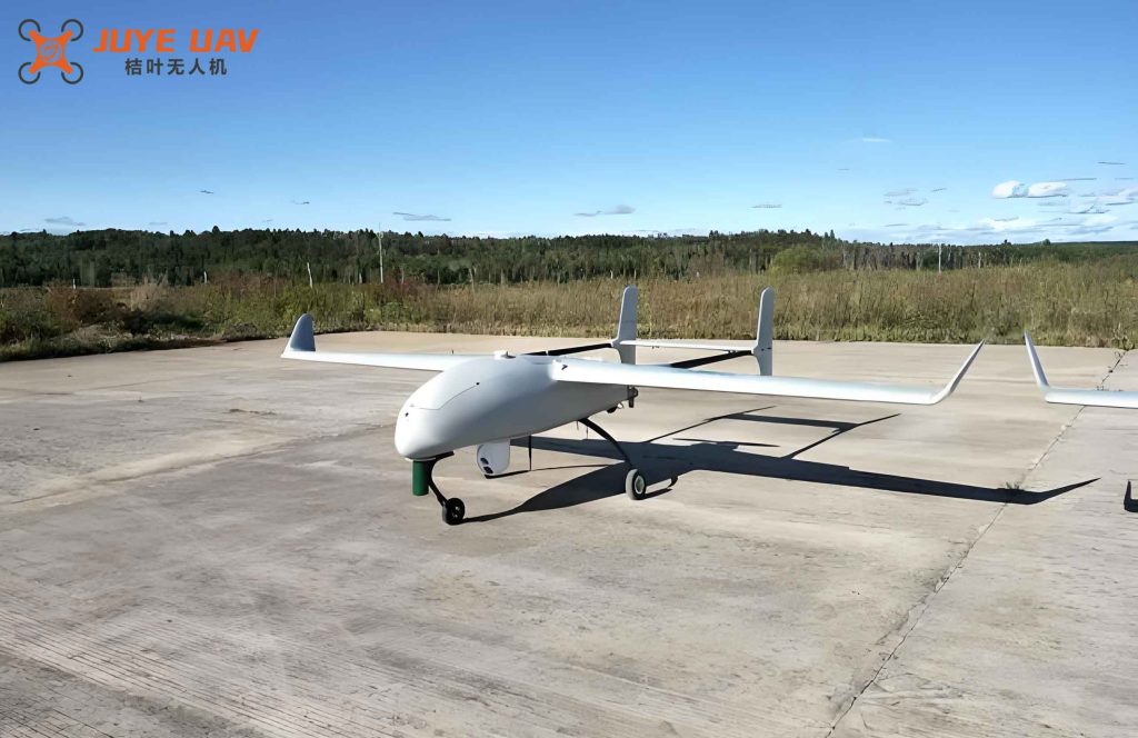
1. Introduction
The maneuverability and endurance of fixed-wing drones make them ideal for long-range missions such as surveillance, reconnaissance, and cargo delivery. In many scenarios, multiple fixed-wing drones operate in formation to achieve collective objectives. Formation path-following requires each drone to track a pre-planned path while maintaining a prescribed relative geometry. However, the underactuated nature of fixed-wing drones—controlled primarily through normal acceleration—poses challenges for accurate tracking, especially when paths contain sharp turns or curvature changes. Current approaches can be broadly categorized into model predictive control, sliding mode control, vector field methods, and virtual structure methods. While these methods perform well on straight-line segments or simple arcs, they often exhibit degraded performance on complex paths with varying curvature. Some methods, such as the front-positioned moving-target approach, align naturally with the lateral acceleration dynamics of a fixed-wing drone, but prior implementations lacked adaptation to path curvature for formation flights. In this work, we propose an enhanced moving-target guidance method that explicitly accounts for path curvature when computing follower target distances, thereby achieving superior lateral precision and zero steady-state error on arcs of constant curvature. We provide a Lyapunov-based stability analysis and validate the method through extensive simulations.
2. Problem Formulation
2.1 Dynamics of a Fixed-Wing Drone
We consider the motion of a fixed-wing drone in the horizontal plane. Neglecting altitude changes, the state variables are the inertial position \(\mathbf{P} = [x, z]^T\), speed \(v\), and heading angle \(\psi\). The control inputs are the forward acceleration \(a_A\) (along the velocity vector) and the normal acceleration \(a_N\) (perpendicular to velocity). The kinematic equations are:
$$
\begin{aligned}
\dot{x} &= v\cos\psi, \\
\dot{z} &= -v\sin\psi, \\
\dot{v} &= a_A, \\
\dot{\psi} &= \frac{a_N}{v}.
\end{aligned}
$$
The normal acceleration is the primary control for turning, generated by banking the fixed-wing drone to produce a horizontal component of lift. This underactuated characteristic motivates guidance laws that directly command \(a_N\) based on a geometric construction such as the moving-target logic.
2.2 Formation Definition
We define a formation coordinate system (FCS) with origin at the leader’s position \(\mathbf{P}_0\) and orientation aligned with the leader’s velocity direction. The FCS axes are denoted \(X_F\) (along the leader’s velocity) and \(Z_F\) (perpendicular to the right). A follower’s desired position in FCS is given by \(\mathbf{P}_{i,d,F} = [x_{i,d,F}, z_{i,d,F}]^T\). The transformation from inertial coordinates to FCS is:
$$
\begin{bmatrix} x_F \\ z_F \end{bmatrix} =
\begin{bmatrix} \cos\psi_0 & -\sin\psi_0 \\ \sin\psi_0 & \cos\psi_0 \end{bmatrix}
\begin{bmatrix} x – x_0 \\ z – z_0 \end{bmatrix}.
$$
The control objective is to design commands \(a_N\) and \(a_A\) for each fixed-wing drone such that the leader follows the given path \(s\) precisely, and each follower maintains its desired position in FCS (i.e., the formation is preserved).
3. Proposed Guidance Method
3.1 Single Fixed-Wing Drone Path-Following
We first develop a guidance law for a single fixed-wing drone to follow a planar curve \(s\). As illustrated in Figure 1 (conceptual), let \(D\) be a fixed look-ahead distance. We draw a circle of radius \(D\) centered at the drone’s position. The intersection of this circle with the path, when the drone is sufficiently close to the path, yields two points. We choose the point ahead along the path as the moving target point \(\mathbf{T}_0\). If there is no intersection, we expand the circle until it is tangent to the path, and then use the intersection of the original circle with the line joining the drone and the tangent point. Once \(\mathbf{T}_0\) is determined, we construct a command arc that passes through the drone position \(\mathbf{P}_0\) and \(\mathbf{T}_0\), with the tangent at \(\mathbf{P}_0\) aligned with the drone’s velocity. The radius \(R\) of this arc is given by:
$$
R = \frac{D}{2\cos\eta_0},
$$
where \(\eta_0\) is the angle between the velocity and the line \(\mathbf{P}_0\mathbf{T}_0\). The required normal acceleration command is the centripetal acceleration of the arc:
$$
a_{Nc0} = \frac{2v_0^2 \cos\eta_0}{D} = \frac{2v_0^2 \sin q_0}{D},
$$
with \(q_0\) being the target line-of-sight angle. This law guides the drone onto the path with zero steady-state error when the path curvature is constant, because at equilibrium the command arc coincides with the path, and the required acceleration matches the ideal turning acceleration. The leader uses this law to track the reference path.
3.2 Multi-Drone Formation Path-Following
For formation flight, we adopt a leader-follower architecture. The leader executes the single-drone path-following law. Each follower (index \(i>0\)) also uses a similar moving-target logic, but its target point is computed from the leader’s target point and the desired formation position. Let \(\mathbf{T}_0\) be the leader’s moving target, and \(\psi_{T0}\) the tangent direction of the path at \(\mathbf{T}_0\). We define a target coordinate system (TCS) with origin at \(\mathbf{T}_0\) and axes aligned with the tangent and normal of the path. The follower’s target point in TCS is set equal to its desired formation position in FCS:
$$
\mathbf{T}_{i,T} = \mathbf{P}_{i,d,F} = [x_{i,d,F}, z_{i,d,F}]^T.
$$
Transforming back to inertial coordinates:
$$
\mathbf{T}_i = \mathbf{L}_T^{-1} \mathbf{P}_{i,d,F} + \mathbf{T}_0,
$$
where \(\mathbf{L}_T\) is the rotation matrix from TCS to inertial. This produces a target formation that moves with the path, preserving the relative geometry even during turns.
Each follower then applies the single-drone guidance law with its own target \(\mathbf{T}_i\), obtaining a normal acceleration command:
$$
a_{Nci} = \frac{2v_i^2 \cos\eta_i}{D_i} = \frac{2v_i^2 \sin q_i}{D_i},
$$
where \(D_i = \|\mathbf{T}_i – \mathbf{P}_i\|\). This command ensures that the follower converges to its moving target, which in turn tracks the path at a desired offset.
3.3 Longitudinal Control via Adaptive Target Distance
The distance \(D_i\) is not fixed; we adjust the desired value \(D_{i,d}\) based on the path curvature to achieve zero steady-state lateral error. For a constant-curvature path of radius \(R_0\), the follower’s path radius is \(R_i = R_0 + z_{i,d,F}\). The ratio of distances should equal the ratio of radii to maintain the same look-ahead geometry:
$$
\frac{D_{i,d}}{D} = \frac{R_i}{R_0}.
$$
Thus, the desired distance is:
$$
D_{i,d} = D \frac{R_0 + z_{i,d,F}}{R_0}.
$$
For straight paths (\(R_0 \to \infty\)), \(D_{i,d} = D\). A low-level target distance controller (e.g., a PID controller) adjusts the forward acceleration \(a_A\) to drive \(D_i\) to \(D_{i,d}\). This adaptive mechanism accounts for the fact that inner (outer) followers need a smaller (larger) look-ahead distance to maintain the same angular offset on curved paths. It eliminates the steady-state error present in previous moving-target methods.
3.4 Algorithm Summary
The overall procedure for each fixed-wing drone is summarized in the table below. The leader uses Algorithm 1 (single drone tracking). Each follower uses Algorithm 2, which incorporates the adaptive target distance.
| Step | Action |
|---|---|
| 1 | Receive leader target \(\mathbf{T}_0\) and path tangent \(\psi_{T0}\). Obtain path curvature radius \(R_0\) (averaged over a segment). |
| 2 | Compute rotation matrix \(\mathbf{L}_T^{-1}\) from \(\psi_{T0}\). |
| 3 | Compute follower target \(\mathbf{T}_i = \mathbf{L}_T^{-1} \mathbf{P}_{i,d,F} + \mathbf{T}_0\). |
| 4 | Measure distance \(D_i = \|\mathbf{T}_i – \mathbf{P}_i\|\) and angle \(q_i\) between velocity and line to target. |
| 5 | Compute normal acceleration command \(a_{Nci} = 2v_i^2 \sin q_i / D_i\). |
| 6 | Compute desired distance \(D_{i,d} = D (R_0 + z_{i,d,F}) / R_0\). |
| 7 | Use target distance controller to compute forward acceleration \(a_{Aci}\) to track \(D_{i,d}\). |
4. Stability Analysis
We analyze the stability of the proposed method for a fixed-wing drone flying on a constant-curvature path. Consider a follower that has already converged to the correct formation (small error). We work in a polar coordinate system centered at the path’s center of curvature. Let \(r\) be the radial distance, \(\chi\) the angular position, \(v_n\) the radial velocity (positive outward), and \(v_t\) the tangential velocity. The dynamics are:
$$
\begin{aligned}
\dot{r} &= v_n, \\
\dot{\chi} &= -\frac{v_t}{r}, \\
\dot{v}_t &= a_t – \frac{v_n v_t}{r}, \\
\dot{v}_n &= -a_n – \frac{v_t^2}{r},
\end{aligned}
$$
where \(a_t\) and \(a_n\) are tangential and normal accelerations. At the desired equilibrium, \(r = R_i\) (the follower’s path radius), \(v_n = 0\), and \(v_t = v_i\) (the speed of the follower). The normal acceleration command from our guidance law can be expressed as a function of the error state. Under small-angle approximations, we obtain:
$$
a_{Nci} \approx a_{Nci,0} + K_p e + K_d \dot{e},
$$
where \(e = r – R_i\) is the radial error, \(a_{Nci,0} = v_t^2 / r\) is the feedforward term, and the coefficients are:
$$
K_p = \frac{2 v_t^2 \cos^2 q_{i0}}{D_i^2}, \quad K_d = \frac{2 v_t \cos q_{i0}}{D_i}.
$$
We choose a Lyapunov function:
$$
V = K_p e^2 + v_n^2.
$$
Its derivative along the dynamics is:
$$
\dot{V} = -2 v_n \left[ K_p e + a_n – \frac{v_t^2}{r} \right].
$$
Substituting the approximated command and neglecting higher-order terms yields \(\dot{V} = -2 v_n (K_d v_n + \text{small terms})\). Since \(K_d > 0\) and the higher-order terms become negligible near equilibrium, \(\dot{V} \le 0\) locally, and \(\dot{V}=0\) only when \(v_n=0\) and \(e=0\). Hence, the equilibrium is asymptotically stable. The same reasoning applies to the leader when tracking a constant-curvature path. The analysis confirms that the fixed-wing drone formation converges to the desired geometry on curved paths with zero steady-state error.
5. Simulation Results
5.1 Simulation Setup
We simulate the proposed method using a 3-degree-of-freedom point-mass model of a fixed-wing drone with first-order actuator lags for normal and vertical acceleration (time constants 0.5 s and 0.8 s respectively). The altitude is held constant via a PID controller. The leader’s speed is maintained at 50 m/s. The look-ahead distance is set to \(D = 50\) m. We consider two scenarios: (1) convergence from random initial conditions on a circular path of radius 500 m, and (2) tracking of a complex path composed of multiple arcs and straight lines with curvatures ranging from 500 m to 2000 m radii. In the second scenario, we compare our method (adaptive moving-target) against three alternatives: PID-based position control, vector-field method (based on arctan guidance), and the non-adaptive moving-target approach from prior work. Two followers are placed at lateral offsets of ±100 m.
5.2 Convergence from Random Initial Conditions
Ten followers with random initial positions (\(\pm 100\) m in y, \(\pm 10\) m in x), speeds (45–55 m/s), and headings (\(\pm 45^\circ\)) are commanded to form a line-abreast formation on the circular path. Results show that all followers converge to within 0.5 m of their desired positions in less than 10 s. The adaptive target distance naturally creates speed differences between inner and outer drones, enabling precise formation maintenance without collision. The maximum overshoot in the formation-keeping error remains below 2 m.
| Follower ID | Time to X_F error < 0.5 m (s) | Time to Z_F error < 0.5 m (s) |
|---|---|---|
| 1 | 4.2 | 3.8 |
| 2 | 5.1 | 4.5 |
| 3 | 3.9 | 4.0 |
| 4 | 6.0 | 5.2 |
| 5 | 4.8 | 4.1 |
| 6 | 5.5 | 4.9 |
| 7 | 3.5 | 3.6 |
| 8 | 7.2 | 6.1 |
| 9 | 4.0 | 3.7 |
| 10 | 5.8 | 5.0 |
5.3 Complex Path Tracking and Comparison
The second simulation uses a 300-second path with varying curvature. The leader’s lateral tracking error and the followers’ positions in the formation coordinate system are recorded. The table below summarizes the root-mean-square (RMS) errors and maximum errors for the four methods.
| Method | Leader lateral RMS error (m) | Follower 1 X_F RMS error (m) | Follower 1 Z_F RMS error (m) | Follower 1 max X_F error (m) | Follower 1 max Z_F error (m) |
|---|---|---|---|---|---|
| Adaptive moving-target | 0.08 | 0.79 | 1.76 | 4.04 | 0.10 |
| PID position control | 2.54 | 0.96 | 3.11 | 5.49 | 7.53 |
| Vector-field method | 0.38 | 1.84 | 3.18 | 9.76 | 15.35 |
| Non-adaptive moving-target | 0.08 | 0.79 | 2.23 | 4.04 | 3.35 |
Our adaptive method achieves the smallest lateral error (Z_F direction) for the follower, with RMS error of 1.76 m and maximum error of only 0.10 m (the latter is almost negligible). The non-adaptive moving-target method shows a larger Z_F max error (3.35 m) due to curvature-induced steady-state offsets. PID and vector-field methods exhibit even larger errors, especially during turns. The leader tracking accuracy is also superior for our method and the non-adaptive one (same leader law), outperforming PID and vector field. In the longitudinal direction (X_F), all methods perform similarly because the inner loop dynamics limit performance, but the adaptive method still shows slightly smaller RMS error.
6. Conclusion
We have developed a formation path-following guidance method for fixed-wing drones based on a front-positioned moving-target approach. The key contributions include: (1) a single-drone guidance law that achieves zero steady-state error on constant-curvature paths; (2) an extension to formation flight where follower target points are derived from the leader’s target and desired formation positions, with adaptive target distance based on local path curvature; (3) a Lyapunov-based stability proof for constant-curvature paths; and (4) simulation validation demonstrating improved accuracy and robustness compared to existing methods. Our adaptive method reduces lateral formation errors by an order of magnitude on complex paths, making it particularly suitable for fixed-wing drone swarms operating in narrow corridors or cluttered environments. Future work will incorporate disturbance observers to handle wind gusts and model uncertainties.