
The coordinated flight of multiple unmanned aerial vehicles (UAVs), or drone formation flight, has transcended its initial military applications to become a cornerstone technology for commercial, scientific, and public safety missions. Observing biological systems like migrating geese or schooling fish reveals a profound truth: collective motion is often far more efficient, robust, and capable than individual movement. This principle directly translates to drone formations, where a group of UAVs can perform complex tasks such as large-scale environmental monitoring, search and rescue in disaster zones, or precision agricultural surveying with greater coverage and resilience than a single agent. The advent of modern embedded systems, networked communication, and advanced control theory has made the realization of such sophisticated multi-agent systems increasingly feasible.
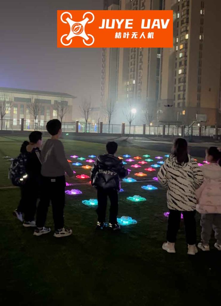
However, the very foundation of a cohesive drone formation relies on reliable information exchange between its members. In real-world scenarios, this communication is perpetually susceptible to disruptions. Factors such as limited communication bandwidth, electromagnetic interference, signal attenuation, and network congestion invariably introduce time delays in the transmission of state information (e.g., position, velocity) between UAVs. These delays are not merely constant or predictable; they are often stochastic in nature, varying randomly with network conditions. Ignoring this reality can lead to degraded performance, oscillatory behavior, or even instability in the drone formation control system. Therefore, developing control strategies that explicitly account for and are robust to stochastic communication delays is not just an academic exercise but a critical necessity for the reliable deployment of autonomous UAV swarms.
Overview of Drone Formation Control Methodologies
Several foundational strategies have been developed to address the multi-agent coordination problem inherent in drone formation control. Each offers a unique perspective and comes with its own set of advantages and challenges, as summarized below.
| Methodology | Core Principle | Advantages | Challenges |
|---|---|---|---|
| Leader-Follower | Designates one or more UAVs as leaders. Followers track the leader’s state with a prescribed offset. | Conceptually simple, easy to implement. | Single point of failure (if leader fails), lack of explicit cooperation among followers. |
| Behavior-Based | Defines a set of basic behaviors (e.g., collision avoidance, goal attraction). The final control input is a weighted sum of behavior-specific controllers. | Intuitive, flexible, handles multiple objectives well. | Formal stability analysis can be difficult; behavior weighting is often heuristic. |
| Virtual Structure | Treats the entire formation as a single rigid virtual body. Each UAV tracks a corresponding point on this virtual structure. | Provides precise geometric formation control, good for rigid patterns. | Less flexible for dynamic formation changes; requires centralized trajectory generation for the virtual structure. |
| Consensus-Based | UAVs update their states based on the relative states of their neighbors. The goal is to achieve agreement (consensus) on states like velocity or heading. | Fully distributed, promotes explicit cooperation, strong theoretical foundation. | The final formation geometry is often defined implicitly by the consensus protocol, requiring careful design for specific patterns. |
In this work, I adopt and extend a strategy that synergizes elements of the consensus-based and virtual structure approaches. The control objective is for a group of $n$ vertical take-off and landing (VTOL) UAVs to achieve and maintain a desired geometric pattern defined by constant relative position vectors $\delta_{ij}$ (where $\delta_{ij} = \delta_i – \delta_j$), while ultimately coming to a hover. Crucially, this must be accomplished despite the presence of random, time-varying delays in the inter-agent communication links.
System Modeling and Problem Formulation
VTOL UAV Dynamics
I consider a fleet of $n$ identical VTOL UAVs (e.g., quadrotors). The dynamics of the $i$-th UAV, where $i \in \mathcal{N} = \{1, …, n\}$, are described by a translation subsystem and a rotation subsystem. The translational dynamics, governing the motion of the center of mass, are given by:
$$
\begin{aligned}
\dot{\mathbf{p}}_i &= \mathbf{v}_i \\
\dot{\mathbf{v}}_i &= \mathbf{F}_i – \frac{\Lambda_i}{m_i} \left( R(\mathbf{Q}_i)^T – R(\mathbf{Q}_{di})^T \right) \mathbf{\hat{e}}_3
\end{aligned}
$$
where $\mathbf{p}_i \in \mathbb{R}^3$ and $\mathbf{v}_i \in \mathbb{R}^3$ are the position and linear velocity vectors expressed in an inertial frame. $\mathbf{F}_i \in \mathbb{R}^3$ is an intermediate virtual control force to be designed. $\Lambda_i \in \mathbb{R}$ is the magnitude of the total thrust force, and $m_i$ is the mass. $R(\mathbf{Q}_i) \in SO(3)$ is the rotation matrix from the body frame to the inertial frame, parameterized by the unit quaternion $\mathbf{Q}_i = (\mathbf{q}_i^T, \eta_i)^T \in \mathbb{S}^3$. $\mathbf{Q}_{di}$ is a desired attitude quaternion, and $\mathbf{\hat{e}}_3 = (0, 0, 1)^T$.
The rotational (attitude) dynamics are:
$$
\begin{aligned}
\dot{\mathbf{Q}}_i &= \frac{1}{2} \mathbf{T}(\mathbf{Q}_i) \boldsymbol{\omega}_i \\
\mathbf{J}_i \dot{\boldsymbol{\omega}}_i &= \boldsymbol{\Gamma}_i – S(\boldsymbol{\omega}_i) \mathbf{J}_i \boldsymbol{\omega}_i
\end{aligned}
$$
Here, $\boldsymbol{\omega}_i \in \mathbb{R}^3$ is the angular velocity in the body frame, $\mathbf{J}_i \in \mathbb{R}^{3 \times 3}$ is the inertia matrix, and $\boldsymbol{\Gamma}_i \in \mathbb{R}^3$ is the control torque input. The matrices $S(\cdot)$ (skew-symmetric) and $\mathbf{T}(\cdot)$ are standard mappings from the quaternion algebra.
The attitude tracking error quaternion $\tilde{\mathbf{Q}}_i = (\tilde{\mathbf{q}}_i^T, \tilde{\eta}_i)^T$ is defined from the desired attitude $\mathbf{Q}_{di}$. A key relationship used in the control derivation is:
$$
\left( R(\mathbf{Q}_i)^T – R(\mathbf{Q}_{di})^T \right) \mathbf{\hat{e}}_3 = \boldsymbol{\Pi}_i \tilde{\mathbf{q}}_i
$$
where $\boldsymbol{\Pi}_i$ is a matrix function of the attitude error. This connects the translational force error to the attitude error $\tilde{\mathbf{q}}_i$.
Modeling Stochastic Communication Delays
The core challenge addressed in this drone formation control design is the stochastic nature of communication delays. I model the information received by UAV $i$ from its neighbor $j$ using a Bernoulli random variable. Let $\lambda(t)$ be a stochastic process obeying the Bernoulli distribution:
$$
\begin{aligned}
\text{Prob}\{\lambda(t) = 1\} &= \mathbb{E}\{\lambda(t)\} = \bar{\lambda} \\
\text{Prob}\{\lambda(t) = 0\} &= 1 – \bar{\lambda}
\end{aligned}
$$
where $\bar{\lambda} \in [0, 1]$ is the known expectation. The neighbor’s position information used in the controller is then:
$$
\mathbf{p}_j^{\text{recv}}(t) = \lambda(t) \mathbf{p}_j(t) + (1 – \lambda(t)) \mathbf{p}_j(t – \tau_{ij}(t))
$$
Thus, $\lambda(t)=1$ corresponds to a perfect, delay-free transmission, occurring with probability $\bar{\lambda}$. $\lambda(t)=0$ corresponds to the reception of a delayed state $\mathbf{p}_j(t – \tau_{ij}(t))$, occurring with probability $1-\bar{\lambda}$. The time delay $\tau_{ij}(t)$ is time-varying but assumed to be bounded, i.e., $0 \le \tau_{ij}(t) \le \tau_{\text{max}}$. This model effectively captures the random occurrence of packet delays in a networked drone formation.
Controller Design for the Stochastic Delay Case
The control architecture is hierarchical. First, a formation controller generates a desired force $\mathbf{F}_i$ for each UAV. From this force, the required thrust magnitude $\Lambda_i$ and the desired attitude $\mathbf{Q}_{di}$ are extracted. Second, an attitude controller generates the torque $\boldsymbol{\Gamma}_i$ to track $\mathbf{Q}_{di}$.
Translational Formation Controller Design
I define the position and velocity tracking errors for UAV $i$ as:
$$
\begin{aligned}
\boldsymbol{\xi}_i &= \mathbf{p}_i – \boldsymbol{\theta}_i – \boldsymbol{\alpha}_i \\
\mathbf{z}_i &= \dot{\boldsymbol{\xi}}_i = \mathbf{v}_i – \dot{\boldsymbol{\theta}}_i – \dot{\boldsymbol{\alpha}}_i
\end{aligned}
$$
where $\boldsymbol{\theta}_i$ and $\boldsymbol{\alpha}_i$ are auxiliary filter states with arbitrary initial conditions. The intermediate control force $\mathbf{F}_i$ is designed as:
$$
\mathbf{F}_i = -k_i^p \boldsymbol{\chi}(\boldsymbol{\theta}_i) – k_i^d \boldsymbol{\chi}(\dot{\boldsymbol{\theta}}_i)
$$
Here, $k_i^p, k_i^d > 0$ are gains, and $\boldsymbol{\chi}(\cdot)$ is a vector saturation function with properties ensuring boundedness. The dynamics of the filter states are:
$$
\begin{aligned}
\ddot{\boldsymbol{\theta}}_i &= \mathbf{F}_i – \mathbf{u}_i \\
\ddot{\boldsymbol{\alpha}}_i &= \mathbf{u}_i – \boldsymbol{\varphi}_i – \frac{\Lambda_i}{m_i} \boldsymbol{\Pi}_i \tilde{\mathbf{q}}_i
\end{aligned}
$$
The term $\mathbf{u}_i = -L_i^p \boldsymbol{\alpha}_i – L_i^d \dot{\boldsymbol{\alpha}}_i$ stabilizes the $\boldsymbol{\alpha}_i$-dynamics. The critical formation control term $\boldsymbol{\varphi}_i$, which handles neighbor interactions and stochastic delays, is designed as:
$$
\boldsymbol{\varphi}_i = -k_i^v \mathbf{z}_i – \sum_{j=1}^{n} k_{ij} \left[ \lambda \boldsymbol{\xi}_{ij}(t) + (1-\lambda) \boldsymbol{\xi}_{ij}(t-\tau_{ij}(t)) \right]
$$
where $k_i^v > 0$ is a damping gain, $k_{ij}$ are the elements of the graph adjacency matrix defining the communication topology, and $\boldsymbol{\xi}_{ij} = \boldsymbol{\xi}_i – \boldsymbol{\xi}_j – \delta_{ij}$ is the relative formation error. This design seamlessly incorporates the stochastic delay model: the controller uses either the current or the delayed neighbor error based on the instant value of the random variable $\lambda(t)$.
Once $\mathbf{F}_i$ is computed, the actual thrust $\Lambda_i$ and desired attitude $\mathbf{Q}_{di}$ are obtained via the following extraction algorithm:
$$
\begin{aligned}
\Lambda_i &= m_i \| g\mathbf{\hat{e}}_3 – \mathbf{F}_i \| \\
\eta_{di} &= \sqrt{\frac{1}{2} + \frac{m_i(g – F_{i,z})}{2\Lambda_i}}, \quad
\mathbf{q}_{di} = \frac{m_i}{2\Lambda_i \eta_{di}} \begin{pmatrix} F_{i,y} \\ -F_{i,x} \\ 0 \end{pmatrix}, \quad
\mathbf{Q}_{di} = \begin{pmatrix} \mathbf{q}_{di} \\ \eta_{di} \end{pmatrix}
\end{aligned}
$$
where $F_{i,z}$ is the third component of $\mathbf{F}_i$. This algorithm ensures the thrust vector is aligned to produce the desired virtual force.
Rotational Attitude Controller Design
To track the desired attitude $\mathbf{Q}_{di}$ (and its associated angular velocity $\boldsymbol{\omega}_{di}$ derived from $\dot{\mathbf{F}}_i$), I define the angular velocity error as $\tilde{\boldsymbol{\omega}}_i = \boldsymbol{\omega}_i – R(\tilde{\mathbf{Q}}_i) \boldsymbol{\omega}_{di}$. The control torque $\boldsymbol{\Gamma}_i$ is designed using a backstepping-inspired approach:
$$
\begin{aligned}
\boldsymbol{\Gamma}_i &= \mathbf{H}_i(\cdot) + \mathbf{J}_i \dot{\boldsymbol{\beta}}_i – k_i^q \tilde{\mathbf{q}}_i – k_i^{\Omega} (\tilde{\boldsymbol{\omega}}_i – \boldsymbol{\beta}_i) \\
\boldsymbol{\beta}_i &= -k_i^{\beta} \tilde{\mathbf{q}}_i
\end{aligned}
$$
The term $\mathbf{H}_i(\cdot)$ compensates for nonlinear Coriolis and coupling terms, while $k_i^q, k_i^{\Omega}, k_i^{\beta} > 0$ are controller gains. This design ensures fast and stable attitude tracking.
Stability Analysis and Delay-Dependent Conditions
The closed-loop stability of the entire drone formation system under stochastic delays is analyzed using Lyapunov-Krasovskii functional methods combined with stochastic analysis. I construct a composite Lyapunov functional candidate $V = V_t + V_k$.
The main functional $V_t$ addresses the translational errors:
$$
V_t = \frac{1}{2}\sum_{i=1}^{n} \left( \mathbf{z}_i^T \mathbf{z}_i + \frac{1}{2}\sum_{j=1}^{n} k_{ij} \boldsymbol{\xi}_{ij}^T \boldsymbol{\xi}_{ij} \right)
$$
An additional term $V_k$ is introduced specifically to handle the delayed state information using Jensen’s inequality:
$$
V_k = \sum_{i=1}^{n} \sum_{j=1}^{n} \frac{k_{ij} \tau_{\text{max}}}{2\varepsilon} \int_{-\tau}^{0} \int_{t+s}^{t} \mathbf{z}_j^T(\rho) \mathbf{z}_j(\rho) d\rho ds
$$
where $\varepsilon > 0$ is a free parameter. Taking the derivative of $V$, employing the dynamics, and using the properties of the expectation operator $\mathbb{E}\{\cdot\}$ for the Bernoulli variable $\lambda$, I arrive at the following sufficient condition for mean-square stability of the drone formation:
$$
\mathbb{E}\{\dot{V}\} \le \sum_{i=1}^{n} -k_i^z \mathbf{z}_i^T \mathbf{z}_i \quad \text{where} \quad k_i^z = k_i^v – \sum_{j=1}^{n} \frac{k_{ij}}{2} \left[ (\bar{\lambda}-1)\varepsilon + \frac{\tau_{\text{max}}^2}{\varepsilon} \right] > 0
$$
This inequality yields the delay-dependent stability condition. For a given communication graph (defining $k_{ij}$), a known delay bound $\tau_{\text{max}}$, and a known probability $\bar{\lambda}$, the control designer must select the damping gain $k_i^v$ and the parameter $\varepsilon$ such that $k_i^z > 0$ for all $i$. Furthermore, the initial force must satisfy $\|\mathbf{F}_i\| < g$ to ensure the extraction algorithm is valid.
If these conditions hold, the analysis proves that:
- $\mathbf{z}_i \rightarrow 0$, implying $\mathbf{v}_i \rightarrow 0$ (the formation comes to a hover).
- $\boldsymbol{\xi}_{ij} \rightarrow 0$, implying $\mathbf{p}_i – \mathbf{p}_j \rightarrow \delta_{ij}$ (the desired geometric formation is achieved).
- $\tilde{\mathbf{q}}_i \rightarrow 0$ and $\tilde{\boldsymbol{\omega}}_i \rightarrow 0$ (attitude is perfectly tracked).
Thus, the multi-UAV system achieves the global asymptotic formation stabilization goal in probability, despite the presence of stochastic communication delays.
Numerical Simulation and Validation
To validate the proposed stochastic delay-tolerant drone formation controller, I conducted a numerical simulation with $n=4$ VTOL UAVs. The goal was to form a square in the horizontal plane with 4-meter sides.
| Parameter | Value |
|---|---|
| UAV Mass ($m_i$) | 3.0 kg |
| UAV Inertia ($\mathbf{J}_i$) | diag(0.13, 0.13, 0.04) kg·m² |
| Formation Vectors ($\delta_i$) | (2,2,0), (-2,2,0), (-2,-2,0), (2,-2,0) meters |
| Max Communication Delay ($\tau_{\text{max}}$) | 0.2 seconds |
| Time-varying Delay | $\tau_{ij}(t) = 0.2|\sin(0.5t)|$ s |
The communication topology was an undirected, connected graph. The controller gains were tuned according to the stability conditions and are listed below:
| Gain | $k_i^v$ | $k_i^p$ | $k_i^d$ | $k_i^{\beta}$ | $k_i^q$ | $k_i^{\Omega}$ | $L_i^p$ | $L_i^d$ |
|---|---|---|---|---|---|---|---|---|
| Value | 3.0 | 1.5 | 1.4 | 50.0 | 80.0 | 80.0 | 1.0 | 1.0 |
The simulation was run for different values of the delay probability expectation $\bar{\lambda}$, representing various network quality scenarios. The results consistently showed successful convergence to the desired square drone formation and hover. The key performance metrics are summarized as follows:
| Scenario ($\bar{\lambda}$) | Final Formation Error (max $||\mathbf{p}_i-\mathbf{p}_j-\delta_{ij}||$) | Settling Time (to within 5% of final error) | Max Velocity Norm During Transient |
|---|---|---|---|
| Always Delayed ($\bar{\lambda}=0$) | < 0.05 m | ~12 s | 1.8 m/s |
| Often Delayed ($\bar{\lambda}=0.5$) | < 0.03 m | ~10 s | 1.6 m/s |
| Mostly On-Time ($\bar{\lambda}=0.75$) | < 0.02 m | ~8 s | 1.5 m/s |
| Perfect Network ($\bar{\lambda}=1.0$) | < 0.01 m | ~7 s | 1.4 m/s |
The results clearly demonstrate the controller’s robustness. Even in the worst-case scenario where communication is always delayed ($\bar{\lambda}=0$), the drone formation successfully converges to the desired square, albeit with a slightly longer settling time and marginally larger transient velocities compared to the delay-free case. As expected, performance improves as the probability of timely data reception increases. This validates that the derived delay-dependent gain condition effectively ensures stability across the entire spectrum of network conditions.
Conclusion and Future Directions
In this work, I have presented a comprehensive solution for the coordinated control of a drone formation operating under realistic, stochastic communication delays. The proposed method addresses the full nonlinear dynamics of VTOL UAVs, moving beyond simplified point-mass models. By explicitly modeling the random occurrence of delays via a Bernoulli process and incorporating this model directly into the distributed controller design, the scheme guarantees asymptotic formation stability provided a set of explicitly computable, delay-dependent conditions on the control gains are met. The stability proof, grounded in Lyapunov-Krasovskii theory and stochastic analysis, provides strong theoretical guarantees. Numerical simulations confirm the controller’s efficacy and robustness across a range of network quality scenarios.
The framework opens several avenues for future research. First, extending the delay model from Bernoulli to a more general Markov chain could capture correlated delay patterns or packet loss. Second, investigating event-triggered communication strategies integrated with this delay-tolerant control could further optimize network bandwidth usage in a drone formation. Finally, experimental validation with a physical fleet of UAVs operating in a controlled but realistic wireless environment would be the ultimate test of this theory’s practical utility, paving the way for truly reliable and resilient autonomous swarms.