
The rapid advancement of communication network technologies has significantly propelled the intelligence level of unmanned aerial vehicles (UAVs). Leveraging their advantages of low cost, small size, and expansive field of view, unmanned drones have found extensive applications in both civilian and military domains, such as collaborative search, electronic warfare, and navigation guidance.
The core of an unmanned drone formation lies in the navigation design of the cooperative system. Moving Horizon Estimation (MHE) technology can be employed to achieve optimal estimation of the state variables in integrated navigation, thereby obtaining high-precision navigation signals. MHE technology maintains the autonomy of a pure inertial navigation system while acquiring various navigation information such as position, velocity, and attitude angles, enhancing the state estimation accuracy for unmanned drones and expanding the dimensionality of state variables, which holds significant importance in both civilian and military fields.
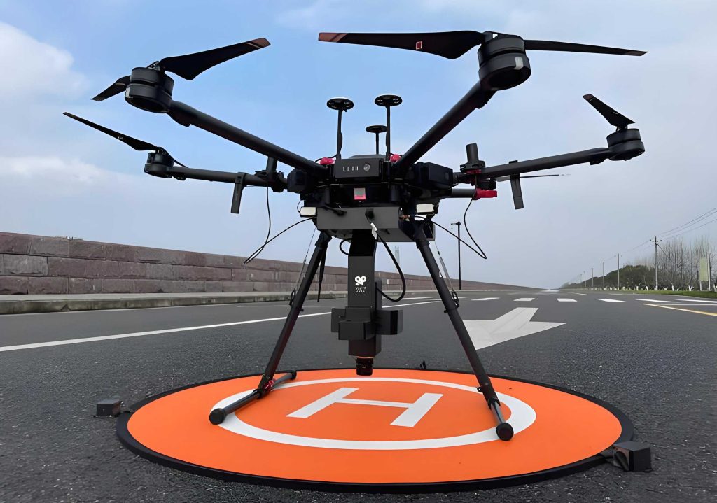
In the realm of state estimation for unmanned drones, substantial research has been conducted in academia. Commonly used methods include Kalman filtering and Moving Horizon Estimation, among others. However, due to factors such as obstructed wireless signals and interference, data transmission between a single unmanned drone’s sensors and controllers may experience packet loss. This paper investigates the state estimation problem concerning the position and velocity of a swarm of unmanned drones. For multi-unmanned drone cooperative systems with feedback control protocols, a Distributed Moving Horizon Estimation (DMHE) algorithm is proposed. This algorithm addresses the packet loss issue by introducing a prediction compensation mechanism and redesigns the cost function within the performance index to analyze the consensus characteristics of the multi-unmanned drone cooperative system’s estimation process. Furthermore, the convergence of the proposed algorithm is analyzed.
1. Problem Formulation and System Modeling
This paper constructs a research scenario based on the context of an unmanned drone formation conducting search and rescue missions inside collapsed buildings after an earthquake. In rescue operations, cooperative unmanned drone systems are deployed to locate missing persons or assess disaster sites. The formation of unmanned drones must navigate through complex rubble and damaged structures, enter narrow and intricate interior spaces, and execute search and rescue actions. This paper considers a formation system composed of $S$ unmanned drones in a Leader-Follower architecture, performing navigation and identification tasks in post-disaster areas. The navigation capability of the unmanned drone formation is crucial for its execution of post-disaster rescue missions, and how to perform accurate real-time estimation of the formation’s state is a key issue for its navigation.
The $S$ unmanned drones take off from different locations at the initial time. The Leader flies according to a reference trajectory, while the remaining unmanned drones adjust their own positions in real-time based on the Leader’s flight state for cooperative flight. During the flight, it is necessary to accurately estimate the states, such as position and velocity, of the unmanned drones to achieve precise positioning and navigation operations.
It is assumed that all $S$ unmanned drones are equipped with networked navigation terminals, enabling them to exchange information with other unmanned drones in the communication network. The network topology among the unmanned drones can be represented by a directed graph $G = (V, E)$, where $V = \{1,2,…,S\}$ and $E \subseteq V \times V$ are the node set and edge set of $G$, respectively. $(i, j) \in E$ indicates that unmanned drone $i$ can communicate with unmanned drone $j$. $\Omega_i = \{j \in V: (i, j) \in E\}$ denotes the set of neighboring unmanned drones for unmanned drone $i$ under the given graph $G$ of the communication network.
The multi-unmanned drone cooperative system considered in this paper is modeled as a set of stochastic linear discrete-time systems:
$$
\begin{align*}
x_{t+1}^{i} &= A x_{t}^{i} + B u_{t}^{i} + \omega_{t}^{i} \\
y_{t}^{i} &= C^{i} x_{t}^{i} + v_{t}^{i}
\end{align*}
$$
where $x^{i} \in \mathbb{R}^{n}$ represents the state variable of unmanned drone $i$, $y^{i} \in \mathbb{R}^{m}$ represents the measurement output of unmanned drone $i$, $u^{i} \in \mathbb{R}^{p}$ represents the control input of unmanned drone $i$, and $\omega^{i}$ and $v^{i}$ represent the system noise and measurement noise, respectively. $A$, $B$, and $C^{i}$ are known system matrices with appropriate dimensions.
The control input of each unmanned drone is influenced by the states of its neighboring unmanned drones. Considering the cooperative relationships among the unmanned drones comprehensively, the cooperative control protocol among them can be given as:
$$
u_{t}^{i} = K x_{t}^{i} + b_{t}^{i} + \sum_{j \in \Omega_i} K (x_{t}^{j} – x_{t}^{i})
$$
where $K \in \mathbb{R}^{p \times n}$ represents the control gain matrix corresponding to information interaction with neighboring unmanned drones, and $b^{i} \in \mathbb{R}^{p}$ represents the reference control input for unmanned drone $i$. Under this control protocol, each interaction between neighboring unmanned drones reflects the cooperative objective of the unmanned drone formation.
Substituting the cooperative control protocol $u_{t}^{i}$ into the system equation, the state evolution of unmanned drone $i$ can be represented as the following dynamic equation:
$$
x_{t+1}^{i} = (A + |\Omega_i| K) x_{t}^{i} + B b_{t}^{i} + B K \sum_{j \in \Omega_i} (x_{t}^{j} – x_{t}^{i}) + \omega_{t}^{i}
$$
where $|\Omega_i|$ is the cardinality of $\Omega_i$.
During the execution of the rescue mission, the unmanned drone formation is interconnected via a wireless communication network to share location information, status data, and target information. However, factors such as damaged power facilities after an earthquake may hinder radio wave propagation, leading to packet loss phenomena. Rescue operations often rely on real-time data feedback for rapid strategy adjustment, and packet loss can result in the absence of critical information, thereby affecting rescue effectiveness. Therefore, it is necessary to design a packet loss compensation algorithm to repair the data incompleteness caused by packet loss in real-time. This paper proposes a prediction compensation strategy to compensate for data loss, using a random variable $\gamma_t$ to express the packet loss phenomenon. The random variable $\gamma_t$ follows a Bernoulli distribution, taking values of 0 or 1. $\gamma_t = 0$ indicates packet loss at time $t$, and $\gamma_t = 1$ indicates no packet loss at time $t$.
$$
\begin{align*}
P(\gamma_t = 1) &= E\{\gamma_t\} = \bar{\gamma} \\
P(\gamma_t = 0) &= 1 – \bar{\gamma}
\end{align*}
$$
where $P(\cdot)$ denotes probability, and $E\{\cdot\}$ denotes the expectation operator.
Remark 1: The estimator can determine whether packet loss has occurred through network detection methods; therefore, the value of $\gamma_t$ can be directly obtained.
When a data packet is lost, this paper employs an output prediction compensation strategy to mitigate the impact of packet loss. The available effective data at the estimator can then be represented as:
$$
\tilde{y}_{t|k}^{i} = \gamma_t y_{t}^{i} + (1 – \gamma_t) z_{t|k-1}^{i}
$$
where $\tilde{y}_{t|k}^{i}$ represents the output value at time $t$ obtained via the prediction compensation strategy at time $k$, and $z_{t|k-1}^{i}$ represents the prediction compensation value constructed for the packet loss at time $t$ at time $k$:
$$
z_{t|k-1}^{i} = C^{i} \hat{x}_{t|k-1}^{i}
$$
where $\hat{x}_{t|k-1}^{i}$ represents the predicted state estimate for time $t$ at time $k-1$.
In summary, the system model for unmanned drone $i$ can be represented as:
$$
\begin{align*}
x_{t+1}^{i} &= (A + |\Omega_i| K) x_{t}^{i} + B b_{t}^{i} + B K \sum_{j \in \Omega_i} (x_{t}^{j} – x_{t}^{i}) + \omega_{t}^{i} \\
\tilde{y}_{t|k}^{i} &= \gamma_t (C^{i} x_{t}^{i} + v_{t}^{i}) + (1 – \gamma_t) C^{i} \hat{x}_{t|k-1}^{i}
\end{align*}
$$
Equation (7) embodies the coupling relationship among the unmanned drones. When a multi-unmanned drone system performs formation navigation tasks, the states and behaviors of individual unmanned drones influence each other.
2. Design of the Distributed Moving Horizon Estimator
For the target unmanned drone $i$, it first interacts with its neighboring unmanned drones. Then, the state predictions from the neighbors and the observation from the target unmanned drone are transmitted to the Moving Horizon Estimator, which ultimately computes the optimal state estimate for unmanned drone $i$. The operational process is illustrated in Figure 1.
When an unmanned drone formation executes rescue missions, multiple unmanned drones need to process data cooperatively via the network. However, factors such as collapsed buildings post-disaster, unstable signal transmission, and significant communication delays between unmanned drones can cause data asynchrony among them, leading to a lack of state consensus. This can result in chaotic formations, affecting overall flight coordination and reducing rescue efficiency.
Therefore, this paper employs a consensus algorithm to address the aforementioned problem. Drawing from the literature, within the Moving Horizon Estimation framework, the cost function in the performance index is reconstructed as a fused cost function, which is the weighted average of the local arrival cost of the target unmanned drone and the local arrival costs of its neighboring unmanned drones. A weighted fusion consensus algorithm for state estimates is also provided. Based on the above analysis, the state estimate for the target unmanned drone can be obtained by solving the following optimization problem:
$$
\min_{\hat{x}_{t-N|t}^{i}} J_t^i
$$
with the cost function $J_t^i$ defined as:
$$
J_t^i = \mu_i \|\hat{x}_{t-N|t}^{i} – \bar{x}_{t-N}^{i}\|_{P_{t-N}^i}^2 + \sum_{j \in \Omega_i} \mu_j \|\hat{x}_{t-N|t}^{i} – \hat{x}_{t-N|t}^{j}\|_{P_{t-N}^j}^2 + \sum_{k=t-N}^{t} \|\tilde{y}_{k|t}^{i} – C^i \hat{x}_{k|t}^{i}\|_{R^i}^2
$$
subject to the following constraints:
$$
\begin{align*}
x &\in \mathbb{X} = \{x: \|x\| \leq \theta_x\} \\
v &\in \mathbb{V} = \{v: \|v\| \leq \theta_v\} \\
\omega &\in \mathbb{W} = \{\omega: \|\omega\| \leq \theta_\omega\}
\end{align*}
$$
where $N+1$ is the moving horizon window length, $\mathcal{L} = \{t-N, t-N+1, …, t\}$, $J_t^i$ denotes the performance index of this optimization problem, the weight coefficients $\mu_i > 0$ and satisfy $\mu_i + \sum_{j \in \Omega_i} \mu_j = 1$. The positive definite weight matrix $R^i$ is a parameter to be designed, and it is set as $R^i = r_i I$. The positive definite weight matrix $P_{t-N}^i$ is used to characterize the confidence in the prior estimate $\bar{x}_{t-N}^{i}$.
The first two terms in Equation (8) represent the arrival cost. They summarize the influence of data before time $t-N$ on the current data, and the second term considers the state consensus problem among the unmanned drones. The third term weights the distance between the predicted output and the actual output using the positive definite weight matrix $R^i$.
Furthermore, the state estimate at time $t-N$ can be computed according to:
$$
\bar{x}_{t-N}^{i} = (A + |\Omega_i| K) \hat{x}_{t-N-1|t-1}^{i} + B b_{t-N-1}^{i} + B K \sum_{j \in \Omega_i} (\hat{x}_{t-N-1|t-1}^{j} – \hat{x}_{t-N-1|t-1}^{i})
$$
For other time instants within the moving horizon window, the corresponding state estimates are given by:
$$
\hat{x}_{t-N+\tau|t}^{i} = (A + |\Omega_i| K) \hat{x}_{t-N+\tau-1|t}^{i} + B b_{t-N+\tau-1}^{i} + B K \sum_{j \in \Omega_i} (\hat{x}_{t-N+\tau-1|t}^{j} – \hat{x}_{t-N+\tau-1|t}^{i}), \quad \tau=1,…,N
$$
In summary, by solving the optimization problem in Equation (8) at time $t$, the optimal state estimation result $\hat{x}_{t-N|t}^{i*}$ for the unmanned drone can be obtained.
3. Estimator Performance Analysis
To facilitate the analysis of the estimator’s performance, the estimation error for unmanned drone $i$ at time $t-N$ is defined as:
$$
e_{t-N}^{i} = x_{t-N}^{i} – \hat{x}_{t-N|t}^{i*}
$$
Denote $\bar{A} = A + |\Omega_i| K$ and $\bar{B} = B K$. By recursively applying Equation (7) within a moving horizon window of length $N$, and stacking the outputs, neighbor states, compensation terms, and noise terms chronologically, the output vector of the target unmanned drone within the window can be written in a unified matrix form:
$$
Y_t^i = \Xi_N^i F_N^i x_{t-N}^{i} + \Xi_N^i G_N^i \sum_{j \in \Omega_i} X_t^j + \Xi_N^i S_N^i b_t^i + \Xi_N^i H_N^i W_t^i + V_t^i + \bar{\Xi}_N^i F_N^i \hat{x}_{t-N|t-1}^{i} + \bar{\Xi}_N^i G_N^i \sum_{j \in \Omega_i} \hat{X}_t^j + \bar{\Xi}_N^i S_N^i b_t^i
$$
where $Y_t^i$ denotes the window output vector composed of $y_{t-N}^{i}$ to $y_t^{i}$; $X_t^j$ denotes the stacked state vector of neighboring unmanned drone $j$ within the window; $W_t^i$ and $V_t^i$ represent the stacked vectors of process noise and measurement noise, respectively; $\Xi_N^i$ and $\bar{\Xi}_N^i$ are diagonal selection matrices formed jointly by the packet loss variables and the prediction compensation terms; $F_N^i$, $G_N^i$, $S_N^i$, $H_N^i$ are the state propagation matrix, neighbor coupling matrix, compensation input matrix, and noise propagation matrix obtained after recursive expansion, respectively.
To ensure consistency between the theoretical analysis and the engineering scenario, the following assumptions are made:
Assumption 1: Under the constraints of the mission flight envelope, control input limits, and onboard sensor measurement ranges, the system state, process noise, measurement noise, and prediction compensation residuals are all bounded. Therefore, the true state $x_t$ always belongs to the convex set $\mathbb{X}$.
Assumption 2: Under the given communication topology, the local cooperative subsystem constituted by the target unmanned drone and its neighboring unmanned drones satisfies overall observability within the moving horizon window.
Assumption 1 aligns with the post-disaster complex environment formation search and rescue scenario considered in this paper. Unmanned drones need to fly inside collapsed buildings, where their position, velocity, and control inputs are constrained by both the flight control system and the mission space. Additionally, the operational ranges of networked navigation terminals and onboard sensors are limited, and abnormal measurements are suppressed by preprocessing stages; thus, considering the state and disturbances as bounded is reasonable. Assumption 2 indicates that, although the post-disaster building environment introduces occlusion, fading, and random packet loss, as long as the formation communication topology remains connected within the estimation window and the target unmanned drone can continuously obtain its own measurements and some neighbor state information, the system can still maintain observability relying on temporal accumulation of observations and fusion of neighbor information. This condition provides the necessary foundation for the subsequent convergence analysis of the distributed estimator.
Supported by the above assumptions and related definitions, theoretical results regarding the convergence of the estimator can be established.
Theorem 1: For the aforementioned system model (7) and error form (11), if there exist two positive definite matrices $P_{t-N}^i$ and $R^i$ such that:
$$
\delta = 4 \sigma_{\text{max}} (\bar{A}^T \bar{A}) < 1
$$
then the mean-square value limit of the unmanned drone estimation error converges to an upper bound:
$$
\lim_{t \to \infty} E\{ \| e_{t-N}^{i} \|^2 \} \leq \frac{c}{1 – \delta}
$$
Proof: To complete the proof of this theorem, it is necessary to bound the range of the minimum value of the performance index. By the optimality principle of $\hat{x}_{t-N|t}^{i*}$, an upper bound for the minimum value $J_t^{i*}$ of Equation (8) can be derived. Substituting the stacked output relation of Equation (12) into the second term of Equation (15) and scaling the noise terms, compensation residual terms, and neighbor coupling terms yields:
$$
J_t^{i*} \leq \mu_i \| x_{t-N}^{i} – \bar{x}_{t-N}^{i} \|_{P_{t-N}^i}^2 + \sum_{j \in \Omega_i} \mu_j \| x_{t-N}^{i} – \hat{x}_{t-N|t}^{j} \|_{P_{t-N}^j}^2 + \varphi_1
$$
where $\varphi_1$ is a positive constant formed jointly by the window length $N$, the upper bounds of process noise, measurement noise, and compensation error.
Next, a lower bound for the minimum value $J_t^{i*}$ of the performance index is analyzed. After similar manipulations and scaling, a lower bound for $J_t^{i*}$ can be obtained as:
$$
J_t^{i*} \geq \lambda_{\text{min}}(P_{t-N}^i) \| e_{t-N}^{i} \|^2 – \varphi_2 \| x_{t-N}^{i} – \bar{x}_{t-N}^{i} \| – \varphi_3
$$
Combining the upper and lower bounds yields:
$$
\lambda_{\text{min}}(P_{t-N}^i) \| e_{t-N}^{i} \|^2 \leq \mu_i \| x_{t-N}^{i} – \bar{x}_{t-N}^{i} \|_{P_{t-N}^i}^2 + \sum_{j \in \Omega_i} \mu_j \| x_{t-N}^{i} – \hat{x}_{t-N|t}^{j} \|_{P_{t-N}^j}^2 + \varphi_1 + \varphi_2 \| x_{t-N}^{i} – \bar{x}_{t-N}^{i} \| + \varphi_3
$$
Furthermore, we have the relationship:
$$
\| x_{t-N}^{i} – \bar{x}_{t-N}^{i} \| \leq \| \bar{A} \| \cdot \| e_{t-N-1}^{i} \| + \varphi_4
$$
Substituting this into the inequality and applying the Young’s inequality, we obtain:
$$
\| e_{t-N}^{i} \|^2 \leq \delta \| e_{t-N-1}^{i} \|^2 + c
$$
where $\delta = 4 \sigma_{\text{max}} (\bar{A}^T \bar{A})$ and $c$ is a positive constant aggregating $\varphi_1, \varphi_2, \varphi_3, \varphi_4$. Taking the expectation on both sides gives:
$$
E\{ \| e_{t-N}^{i} \|^2 \} \leq \delta E\{ \| e_{t-N-1}^{i} \|^2 \} + c
$$
If $\delta < 1$, iterating this inequality leads to:
$$
\lim_{t \to \infty} E\{ \| e_{t-N}^{i} \|^2 \} \leq \frac{c}{1 – \delta}
$$
Thus, Theorem 1 is proven. The convergence analysis shows that, under common conditions of bounded system disturbances and measurement noise, the proposed Distributed Moving Horizon Estimation algorithm can ensure the convergence of the estimation error for the system corresponding to Equation (7).
4. Simulation Verification and Discussion
To validate the effectiveness of the Moving Horizon Estimation algorithm proposed in this paper, a formation system consisting of four unmanned drones is considered. In the simulation environment, Unmanned Drone 4 acts as the leader, flying according to a reference trajectory, while the remaining unmanned drones adjust their positions in real-time based on the leader’s flight state for cooperative flight. The coupling relationship among the unmanned drones is shown in Figure 2.
Selecting the model of any unmanned drone $i$ in the networked navigation system, its parameters are as follows:
$$
A = \begin{bmatrix}
1 & 0 & T_s & 0 \\
0 & 1 & 0 & T_s \\
0 & 0 & 1 & 0 \\
0 & 0 & 0 & 1
\end{bmatrix}, \quad K = \begin{bmatrix}
-0.22 & -0.47 & 0 & 0 \\
0 & 0 & -0.22 & -0.47
\end{bmatrix}
$$
$$
B = \begin{bmatrix}
\frac{T_s^2}{2} & 0 \\
0 & \frac{T_s^2}{2} \\
T_s & 0 \\
0 & T_s
\end{bmatrix}, \quad C^i = \begin{bmatrix}
1 & 0 & 0 & 0 \\
0 & 1 & 0 & 0 \\
0 & 0 & 1 & 0 \\
0 & 0 & 0 & 1
\end{bmatrix}
$$
The sampling time is denoted as $T_s$, taken as $1$ second in the experiment. The number of unmanned drones is $S=4$. The moving horizon estimation window size is 4, the number of simulation runs is $m=100$, $P_0 = 4I$, $R=4I$, $Q=15$, $\mu_1=0.53$, $\mu_2=0.2$, $\mu_3=0.18$, $\mu_4=0.09$. The packet loss probability $\bar{\gamma}$ is set to 0.2. The initial states are set as:
$x_0^1 = [2, 2, 1, 2]^\top$, $x_0^2 = [3, 3, 2, 3]^\top$, $x_0^3 = [4, 4, 3, 4]^\top$, $x_0^4 = [1, 2, 2, 1]^\top$.
Let $x_t^i = [x_{1,t}^i, x_{2,t}^i, x_{3,t}^i, x_{4,t}^i]^\top$ represent the state vector of unmanned drone $i$ at time $t$, sequentially denoting the position in the x-direction, velocity in the x-direction, position in the y-direction, and velocity in the y-direction.
The algorithm performance is measured using the Root Mean Square Error (RMSE), calculated as:
$$
\text{RMSE}_k = \sqrt{\frac{1}{m} \sum_{i=1}^{m} \| x_k^i – \hat{x}_k^i \|^2 }
$$
The simulation results based on the Moving Horizon Estimation algorithm are shown in Figures 3-11.
Analyzing the state trajectory plots for Unmanned Drones 1 through 4 (Figures 3-6), it can be observed that the proposed method can accurately estimate the position and velocity states of the unmanned drones. The deviation between the estimated values and the true values gradually approaches zero, thereby validating the effectiveness of the proposed distributed estimation algorithm.
Figure 7 illustrates the impact of different compensation strategies on estimation performance. The simulation results show that after 100 sampling instants, the steady-state RMSE of the prediction compensation strategy is reduced by an average of 32.6% compared to the zero-order hold strategy, demonstrating higher estimation accuracy. This indicates that the prediction compensation strategy can more effectively compensate for the performance degradation caused by data packet loss.
This paper employs Absolute Error (ABS) to assess the consensus of the unmanned drone formation in position and velocity states. The ABS at time $t$ is defined as:
$$
\text{ABS}_t = \sum_{i=1}^{S-1} \| x_t^{i} – x_t^{i+1} \|
$$
Figure 8 presents the relative state changes of the unmanned drone formation in the x and y directions for both position and velocity. Figure 9 shows the absolute error trajectories for the four states of the unmanned drone formation. It can be seen that as the sampling instants progress, the absolute errors for position and velocity in both the x and y directions converge to constant values. This indicates that the relative positions of the four unmanned drones remain constant, and their relative velocities approach zero, meaning the unmanned drone formation achieves a consensus state. Figure 10 displays the flight trajectories of the unmanned drone formation and the reference trajectory in two-dimensional space, intuitively showing the flight performance of the formation and indicating that the proposed algorithm has good practical application value.
After conducting 100 sampling simulations of the system and performing statistical analysis on the obtained estimation results, it is found that under random packet loss conditions, the proposed DMHE method exhibits faster error convergence speed compared to the EKF baseline algorithm, and the steady-state RMSE is reduced by an average of 22.9%. As shown in Figure 11, this result indicates that in a network environment with packet loss, the DMHE method combined with a prediction compensation strategy can reconstruct the actual state of the unmanned drones more accurately than the EKF baseline algorithm, which does not incorporate a specialized packet loss compensation mechanism. It should be noted that this performance improvement stems from the combined effect of the moving horizon optimization framework and the packet loss compensation strategy. Therefore, this comparison result demonstrates the superior comprehensive estimation performance of the proposed method in packet loss environments, rather than merely indicating that the DMHE structure itself is superior to EKF under all conditions.
5. Conclusion
Addressing the issues of degraded state estimation accuracy and difficulty in maintaining formation consensus for multi-unmanned drone cooperative systems under packet loss constraints, this paper proposed a Distributed Moving Horizon Estimation algorithm. This method introduces a prediction compensation strategy within the Moving Horizon Estimation framework to compensate for lost data packets and reconstructs the cost function by incorporating interaction information between the target unmanned drone and its neighbors, achieving distributed state estimation for the multi-unmanned drone cooperative system. Concurrently, an estimation error model was established, and the convergence of the proposed algorithm was theoretically analyzed.
Simulation results for a four-unmanned drone formation show that under random packet loss conditions with a probability of 0.2, after 100 sampling instants, the steady-state Root Mean Square Error (RMSE) using the prediction compensation strategy is reduced by an average of 32.6% compared to the zero-order hold strategy; compared to the Extended Kalman Filter (EKF) algorithm, the steady-state RMSE of the proposed algorithm is reduced by an average of 22.9%, with faster error convergence. Furthermore, the absolute errors for the formation’s position and velocity in both the x and y directions gradually converge to stable values, indicating that the relative positions of the individual unmanned drones can be maintained constant and their relative velocities approach zero, effectively sustaining formation consensus.
In summary, the proposed method not only improves the state estimation accuracy of multi-unmanned drone cooperative systems in random packet loss environments but also enhances the consensus maintenance capability during formation flight, providing an effective state estimation approach for multi-unmanned drone cooperative navigation in complex environments. The performance of the proposed DMHE algorithm under various conditions is summarized in the table below.
| Condition / Metric | Proposed DMHE (Prediction Compensation) | DMHE (Zero-Order Hold) | EKF Baseline |
|---|---|---|---|
| Steady-State RMSE (Avg. Reduction) | Baseline (Best Performance) | +32.6% higher than proposed | +22.9% higher than proposed |
| Error Convergence Speed | Fastest | Slower | Slowest |
| Formation Consensus Maintenance | Effective (ABS converges) | Moderate | Poorer under packet loss |
| Key Mechanism | MHE + Prediction Compensation + Consensus Cost | MHE + Simple Hold | Recursive filtering without explicit compensation |
The key formula for the state update within the estimation window, combining neighbor information, is:
$$
\hat{x}_{k+1|t}^{i} = \bar{A} \hat{x}_{k|t}^{i} + B b_{k}^{i} + \bar{B} \sum_{j \in \Omega_i} (\hat{x}_{k|t}^{j} – \hat{x}_{k|t}^{i}), \quad k \in [t-N, t-1]
$$
And the core convergence condition derived from the analysis is $\delta = 4 \sigma_{\text{max}} (\bar{A}^T \bar{A}) < 1$, ensuring bounded mean-square error for the cooperative unmanned drone network.