
With the rapid advancement of smart cities, traffic congestion has become a critical bottleneck for urban efficiency. Traditional fixed roadside units cannot achieve full coverage of complex road networks. China UAV drones, with their high mobility and aerial perspective, serve as flexible mobile sensing nodes, providing real-time multi-dimensional data for traffic emergency management. However, existing UAV crowdsensing (UCS) research often treats sensing accuracy and resource consumption separately, ignoring their strong coupling. We propose a Coupled Gain-Resource Deep Q-Network (CGR-DQN) dynamic scheduling method that explicitly integrates multimodal fusion gain with physical resource consumption into a unified optimization framework. Our framework is specifically designed to address the challenges faced by China UAV drones operating in dynamic urban environments, where the trade-off between sensing quality and energy efficiency is critical.
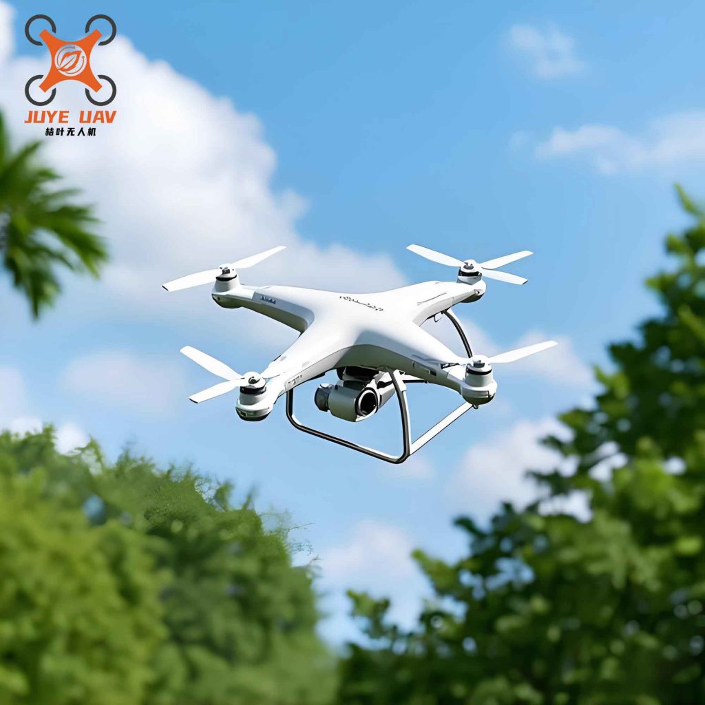
The image below illustrates a typical deployment scenario of China UAV drones for urban traffic sensing.
1. Introduction
China UAV drones are increasingly used in crowdsensing tasks due to their flexible deployment and wide coverage. However, existing research focuses separately on either resource allocation or multimodal fusion. On one hand, resource planning studies aim to minimize energy and latency under communication constraints, treating sensing tasks as generic computational loads. On the other hand, multimodal fusion studies improve detection accuracy under adverse conditions but assume unlimited resources. The reality is that high-fidelity fusion (e.g., RGB + LiDAR) incurs significant energy and bandwidth costs. Furthermore, the value of data is environment-dependent: in foggy weather, LiDAR data is more valuable than visual data, and vice versa. This dynamic coupling makes traditional convex optimization or heuristic methods ineffective.
To overcome these limitations, we design a two-tier architecture comprising UAV sensing nodes and a cloud-edge crowdsensing platform. The platform serves as the decision-making agent that dynamically schedules each China UAV drone’s active state and resource level based on real-time traffic flow conditions and node loads. We introduce a marginal gain coefficient to quantify each node’s contribution to the current multimodal fusion accuracy, and a composite reward function that explicitly couples accuracy gain with resource cost. Using deep reinforcement learning (DQN), our intelligent agent learns optimal scheduling policies in a model-free manner, achieving efficient trade-offs between sensing performance and resource consumption in complex dynamic environments.
2. System Architecture and Mathematical Model
2.1 System Overview
We consider a fleet of N China UAV drones, denoted as N = {n1, n2, …, nN}, each equipped with heterogeneous sensors (RGB camera and LiDAR) operating at a fixed altitude H. The drones collect raw traffic data and upload it via 5G links to a cloud-edge platform. The platform performs multimodal fusion (YOLOv8 for vision, PointNet for point clouds) and extracts traffic features. It also acts as the DRL agent that generates scheduling commands (activate/deactivate nodes, set resource levels) based on the current state.
2.2 Fusion Gain Model
We define the multimodal fusion sensing accuracy at time t as Gt, which aggregates the quality of each modality weighted by dynamic confidence coefficients:
$$ G_t(\mathbf{a}_t, \mathbf{X}_t^f) = \sum_{m=1}^{M} \omega_{m,t} \cdot \Phi_m(\mathbf{a}_t, \mathbf{X}_t^f) $$
where M is the number of modalities (e.g., RGB, LiDAR), and Φm (·) is the cumulative sensing quality of modality m. The dynamic weight ωm,t adjusts based on the environmental feature vector Xtf:
$$ \omega_{m,t} = \frac{\exp(\alpha \cdot \xi_m(\mathbf{X}_t^f))}{\sum_{k=1}^{M} \exp(\alpha \cdot \xi_k(\mathbf{X}_t^f))} $$
Here, ξm(·) is a modality confidence estimation function, and α is a smoothing coefficient. This mechanism robustly down-weights corrupted visual data during fog or night.
For a single node n and modality m, the observation quality qm,n is modeled using a Gaussian decay function:
$$ q_{m,n} = \frac{1}{\sqrt{2\pi\sigma^2}} \exp\left(-\frac{||p_n – p_{\text{target}}||^2}{2\sigma^2}\right) \cdot \mathbb{I}(a_{n,t}=1) $$
The cumulative sensing quality for modality m is then computed by combining all active nodes to capture multi-view collaboration:
$$ \Phi_m = 1 – \prod_{n: a_{n,t}=1} (1 – q_{m,n}) $$
To measure the value of each node, we introduce the marginal gain coefficient ηn,t:
$$ \eta_{n,t} = G_t(\mathbf{a}_t | a_{n,t}=1) – G_t(\mathbf{a}_t | a_{n,t}=0) $$
This coefficient captures the incremental contribution of activating node n. Nodes in overlapping coverage have near-zero marginal gain, while nodes providing complementary views yield high values.
2.3 Resource Consumption Model
The total dynamic energy cost Ct depends on the resource level rn,t ∈ {v1, v2, …, vmax} assigned to each node (sampling frequency, transmission bandwidth). The linear energy model is:
$$ C_t(\mathbf{r}_t) = \sum_{n=1}^{N} r_{n,t} \cdot c_n $$
where cn is the unit resource energy coefficient. The overall instantaneous coupled efficiency F(Gt, Ct | Xtf) quantifies the effective sensing gain per unit resource consumption.
2.4 Optimization Problem
We aim to find the optimal joint policy π* = {at, rt} that minimizes the long-term cost while satisfying a minimum fusion accuracy threshold Gth and hardware constraints. The problem is formulated as:
$$ \begin{aligned}
\min_{a_{n,t}, r_{n,t}} & \quad \sum_{t=1}^{T} \sum_{n=1}^{N} r_{n,t} \cdot c_n \\
\text{s.t.} & \quad G_t \geq G_{th} \\
& \quad \sum_{n=1}^{N} r_{n,t} \cdot c_n \leq C_{\max} \\
& \quad \sum_{n=1}^{N} a_{n,t} \leq K \\
& \quad a_{n,t} \in \{0,1\}, \quad r_{n,t} \in \{v_1, v_2, \ldots, v_{\max}\}
\end{aligned} $$
Due to non-convexity and high dynamics, we transform this problem into a Markov decision process (MDP) and solve it via deep reinforcement learning.
3. Proposed CGR-DQN Algorithm
3.1 MDP Formulation
State Space (S): At each time step t, the state st is a tuple:
$$ \mathbf{s}_t = [G_t, \mathbf{L}_t, \mathbf{X}_t^f, \mathbf{H}_t] $$
- Gt: current fusion accuracy (from Equation 1)
- Lt: resource load vector of all nodes
- Xtf: environmental features (traffic density, weather)
- Ht: previous action history (Ht = at-1) to discourage frequent switching
All continuous values are min-max normalized to [0,1].
Action Space (A): The combined action is At = [at, rt], where at ∈ {0,1}N indicates activation decisions and rn,t selects from discrete resource levels. An action masking mechanism enforces the maximum concurrent node constraint ∑an,t ≤ K.
Reward Function (R): We design a composite reward that explicitly couples gain and cost:
$$ R_t = \mu_1 \log(1 + G_t) + \lambda \sum_{n=1}^{N} \eta_{n,t} – \mu_2 \frac{C_t}{C_{\max}} – \beta \Psi(G_t) $$
where Ψ(Gt) = max(0, Gth – Gt). The logarithmic term models diminishing returns; the marginal gain term encourages activating high-value nodes; the cost term penalizes resource waste; the penalty term ensures satisfaction of the accuracy constraint. We use μ1=0.6, λ=0.2, μ2=0.4, β=10.0.
3.2 Network Architecture and Training
We adopt a DQN architecture with experience replay and double Q-learning. The online network Q(s,a;θ) approximates the action-value function. The target network Q(s,a;θ′) is updated via soft updates (θ′ ← τθ + (1-τ)θ′, τ=0.001). The loss function is:
$$ J(\theta) = \mathbb{E}_{(s,a,r,s’) \sim D} \left[ \left( y – Q(s,a;\theta) \right)^2 \right] $$
where y = r + γ maxa’ Q(s’,a’;θ′) and γ=0.95. The training process is summarized in Algorithm 1.
Algorithm 1 CGR-DQN Training Procedure
| Step | Description |
|---|---|
| 1 | Initialize online network θ, target network θ′ = θ, replay buffer D, exploration rate ε |
| 2 | For each episode k=1..K: |
| 3 | Reset environment, obtain initial state s0 |
| 4 | For t=1..Tmax: |
| 5 | With probability ε choose random action; else at=argmax Q(st,a;θ) |
| 6 | Apply action, observe reward rt and next state st+1 |
| 7 | Store (st, at, rt, st+1) in D |
| 8 | If D has enough samples, sample mini-batch B |
| 9 | Compute yj = rj + γ maxa’ Q(sj+1;θ′) |
| 10 | Update θ via gradient descent on J(θ) |
| 11 | Soft update θ′ ← τθ + (1-τ)θ′ |
| 12 | Decay ε = max(ε_min, ε * decay) |
| 13 | Return trained θ |
4. Experiments and Results
4.1 Experimental Setup
We use the AirV2X dataset (CARLA+AirSim) containing RGB images and LiDAR point clouds from China UAV drones in urban traffic scenarios. Vision features are extracted via YOLOv8, point cloud features via PointNet. The simulation parameters are listed in the table below.
| Parameter | Value |
|---|---|
| Number of drones N | 10 |
| Flight altitude H | 60–100 m |
| Cruise speed | 20 m/s |
| Hover power | 200 W |
| Sensing radius | 80 m |
| Learning rate | 0.0003 |
| Discount factor γ | 0.95 |
| Replay buffer capacity | 50000 |
| Batch size | 64 |
| Soft update coefficient τ | 0.001 |
| Exploration decay rate | 0.995 |
| Accuracy threshold Gth | 0.85 |
| Maximum concurrent nodes K | 5 |
| Max energy per slot Cmax | 20 kW·h |
We compare our CGR-DQN with five baselines: PSO, baseline DQN (without marginal gain and dynamic weights), Actor-Critic (AC), PPO, and Greedy. All DRL methods use the same composite reward function for fairness.
4.2 Convergence Analysis
The average reward convergence curves are shown below. PSO climbs fastest in early episodes but gets stuck at ~55 after 800 episodes. Greedy and AC suffer from high variance. Baseline DQN is limited by lack of dynamic coupling. PPO, as a state-of-the-art on-policy method, reaches ~59 after 1500 episodes. Our CGR-DQN, despite slower start due to ε-greedy exploration, continuously improves and converges to the highest steady reward of ~63 after 1600 episodes, demonstrating that the explicit coupling mechanism effectively guides the agent to a better global optimum.
4.3 Sensing Accuracy and Robustness
We evaluate traffic flow prediction accuracy under different lighting conditions (day, dusk, night) and weather conditions (clear, fog, rain). The table below summarizes the results.
| Scenario | PSO | Baseline DQN | AC | PPO | Greedy | CGR-DQN |
|---|---|---|---|---|---|---|
| Day (clear) | 0.87 | 0.91 | 0.89 | 0.93 | 0.85 | 0.96 |
| Dusk | 0.80 | 0.85 | 0.82 | 0.87 | 0.78 | 0.91 |
| Night | 0.72 | 0.79 | 0.74 | 0.81 | 0.68 | 0.86 |
| Fog | 0.65 | 0.73 | 0.69 | 0.76 | 0.62 | 0.82 |
| Rain | 0.70 | 0.77 | 0.73 | 0.80 | 0.67 | 0.85 |
CGR-DQN outperforms all baselines by 5–10% across all conditions. In foggy weather, our method achieves an accuracy retention rate of 85% (relative to clear day), while others fall below 80%. This is because the dynamic weight mechanism automatically reduces the contribution of degraded visual data and relies more on LiDAR, which is robust to fog. Under packet loss rates of 5%, 10%, and 15%, CGR-DQN’s accuracy degrades by only 2–4%, compared to 8–12% for AC and Greedy.
4.4 Resource Efficiency and Marginal Benefit
We measure comprehensive energy consumption (total energy per task cycle), average CPU utilization of edge nodes, and marginal benefit (ΔG/ΔC). The table below shows the results.
| Metric | PSO | Baseline DQN | AC | PPO | Greedy | CGR-DQN |
|---|---|---|---|---|---|---|
| Energy (kW·h) | 19.8 | 15.2 | 18.5 | 13.8 | 16.4 | 12.6 |
| CPU utilization (%) | 78 | 68 | 72 | 60 | 65 | 55 |
| Marginal benefit | 0.12 | 0.22 | 0.15 | 0.27 | 0.10 | 0.31 |
CGR-DQN achieves the lowest energy (12.6 kW·h) and the highest marginal benefit (0.31). The marginal benefit indicates that each unit of energy invested yields a gain of 0.31 in fusion accuracy, significantly higher than PPO (0.27) and others. This is attributed to the explicit coupling reward that encourages the agent to deactivate low-marginal-gain nodes and assign resources only to where they are most needed. The CPU utilization is also lowest (55%) due to the prior filtering of redundant data.
5. Conclusion
We presented CGR-DQN, a deep reinforcement learning framework that explicitly couples multimodal fusion gain with resource consumption for China UAV drones in smart traffic crowdsensing. By modeling the UCS system as an MDP with a carefully designed composite reward that incorporates marginal gain and resource penalty, our agent learns to dynamically balance sensing accuracy and energy efficiency. Extensive simulations on the AirV2X dataset show that CGR-DQN outperforms PSO, DQN, AC, PPO, and Greedy in terms of convergence, prediction accuracy under various adverse conditions, energy consumption, and marginal benefit. The method demonstrates robust adaptation to communication impairments and weather changes, making it a promising solution for practical deployment of China UAV drones in intelligent transportation systems. Future work will explore federated learning for privacy preservation and extend to GPS-denied environments.