
The coordinated flight of multiple unmanned aerial vehicles (UAVs), or a drone formation, represents a cornerstone technology for modern aerial systems, enabling applications ranging from sophisticated light displays and precision agriculture to complex surveillance and logistical networks. The fundamental challenge initiating any such cooperative mission is the formation forming problem: guiding a group of spatially dispersed drones from arbitrary initial states into a stable, predefined geometric configuration while achieving consensus on their velocity vectors. This paper presents a comprehensive decentralized optimal control framework to address this critical initial phase for a leaderless drone formation with a fixed, undirected communication topology.
Existing methodologies often rely on a leader-follower hierarchy, where the entire drone formation coherence depends on a single agent. This architecture introduces a single point of failure and may not be optimal for scalable, resilient systems. In contrast, our approach empowers each drone to make decisions based solely on information exchanged with its immediate neighbors in the communication graph. This decentralized paradigm enhances the robustness and scalability of the formation. The core of our method involves formulating the formation error relative to neighboring agents, constructing a global performance index amenable to decentralized implementation, and solving for the optimal control law via Linear Matrix Inequalities (LMIs). This ensures that the collective objective of forming a precise drone formation is achieved using only local interactions.
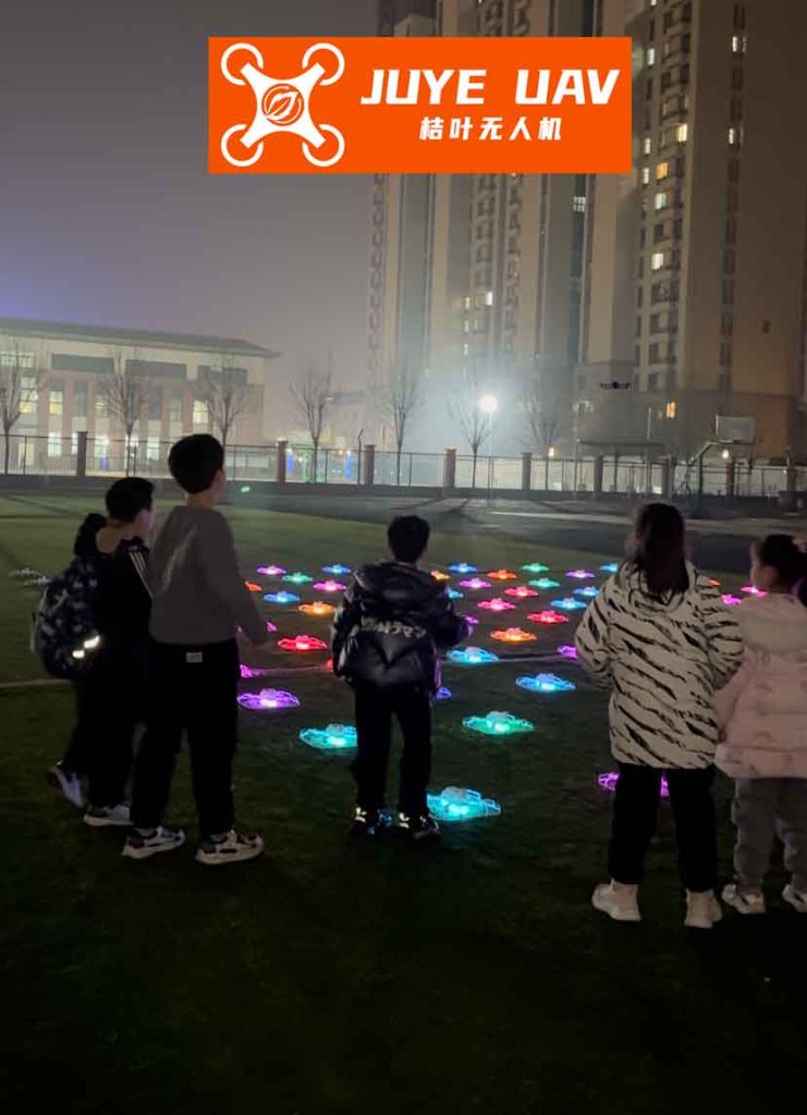
The visual spectacle of a synchronized drone formation light show, as depicted, is a direct manifestation of solved formation control problems. Each drone must know its precise relative position and maintain synchronized motion to create cohesive shapes. The underlying control logic enabling such displays shares fundamental principles with the more general autonomous formation control problem addressed in this research, though often with different performance constraints and objectives.
1. System Modeling and Formation Description
1.1 Agent Dynamics and Linearization
We consider a homogeneous drone formation operating in a planar environment. The kinematics of the i-th drone (UAVi) are commonly modeled as:
$$
\begin{aligned}
\dot{x}_i &= v_i \cos(\theta_i) \\
\dot{y}_i &= v_i \sin(\theta_i) \\
\dot{\theta}_i &= \omega_i \\
\dot{v}_i &= a_i
\end{aligned}
$$
where \((x_i, y_i)\) is the inertial position, \(v_i\) is the speed, \(\theta_i\) is the heading angle, and \(\omega_i\) and \(a_i\) are the angular rate and linear acceleration control inputs, respectively. This model is nonlinear. To apply linear optimal control theory, we adopt a state transformation into a pseudo-linear form. Define the following vectors:
$$
\boldsymbol{\xi}_i = [x_i, y_i, \theta_i, v_i]^T, \quad \boldsymbol{\eta}_i = [a_i, \omega_i]^T
$$
We then define a new state vector \(\mathbf{z}_i\) and a new input vector \(\mathbf{u}_i\):
$$
\mathbf{z}_i = \begin{bmatrix} z_{i1} \\ z_{i2} \\ z_{i3} \\ z_{i4} \end{bmatrix} = \begin{bmatrix} x_i \\ y_i \\ v_i \cos \theta_i \\ v_i \sin \theta_i \end{bmatrix} = \begin{bmatrix} x_i \\ y_i \\ \dot{x}_i \\ \dot{y}_i \end{bmatrix}
$$
$$
\mathbf{u}_i = \begin{bmatrix} \cos(\theta_i) & \sin(\theta_i) \\ -\sin(\theta_i)/v_i & \cos(\theta_i)/v_i \end{bmatrix}^{-1} \boldsymbol{\eta}_i
$$
This yields a linear time-invariant model for each agent:
$$
\dot{\mathbf{z}}_i = A \mathbf{z}_i + B \mathbf{u}_i
$$
with system matrices:
$$
A = \begin{bmatrix} 0 & I_2 \\ 0 & 0 \end{bmatrix}, \quad B = \begin{bmatrix} 0 \\ I_2 \end{bmatrix}
$$
where \(I_2\) is the 2×2 identity matrix. For an n-agent drone formation, the aggregate state and input vectors are \(\mathbf{Z} = [\mathbf{z}_1^T, …, \mathbf{z}_n^T]^T\) and \(\mathbf{U} = [\mathbf{u}_1^T, …, \mathbf{u}_n^T]^T\). The collective dynamics are:
$$
\dot{\mathbf{Z}} = \mathcal{A}_n \mathbf{Z} + \mathcal{B}_n \mathbf{U}
$$
where \(\mathcal{A}_n = I_n \otimes A\) and \(\mathcal{B}_n = I_n \otimes B\), with \(\otimes\) denoting the Kronecker product.
1.2 Communication Topology and Laplacian Matrix
The interaction within the drone formation is defined by a fixed, undirected graph \(\mathcal{G} = (\mathcal{V}, \mathcal{E})\). The vertex set \(\mathcal{V} = \{1, 2, …, n\}\) corresponds to the drones, and the edge set \(\mathcal{E} \subseteq \mathcal{V} \times \mathcal{V}\) represents communication links. If UAVi and UAVj can exchange information, then \((i, j) \in \mathcal{E}\) and \((j, i) \in \mathcal{E}\). The neighborhood of agent \(i\) is \(\mathcal{N}_i = \{j \in \mathcal{V} : (j, i) \in \mathcal{E}, j \neq i\}\).
The topology is encoded in the adjacency matrix \(\mathcal{A}_d = [a_{ij}] \in \mathbb{R}^{n \times n}\), where \(a_{ij} = 1\) if \((j, i) \in \mathcal{E}\) and \(a_{ij}=0\) otherwise. The degree matrix is \(\mathcal{D} = \text{diag}(d_1, …, d_n)\) with \(d_i = \sum_{j=1}^n a_{ij}\). The crucial Laplacian matrix \(\mathcal{L}\) of the graph is defined as:
$$
\mathcal{L} = \mathcal{D} – \mathcal{A}_d
$$
For a connected graph, \(\mathcal{L}\) has a single zero eigenvalue with associated eigenvector \(\mathbf{1}_n\) (the vector of all ones), and all other eigenvalues are positive. This matrix fundamentally governs the diffusion of information and error in the decentralized drone formation control law.
1.3 Desired Formation Geometry
The target drone formation is specified by a constant vector \(\mathbf{h} \in \mathbb{R}^{4n}\). It can be decomposed into position and velocity components:
$$
\mathbf{h} = \mathbf{h}_p \otimes [1, 1, 0, 0]^T
$$
where \(\mathbf{h}_p \in \mathbb{R}^{2n}\) defines the desired relative positions. A stable geometric formation is achieved when there exist vectors \(\mathbf{q}(t) \in \mathbb{R}^2\) and \(\mathbf{w}(t) \in \mathbb{R}^2\) such that:
$$
\lim_{t \to \infty} (\mathbf{Z}_p(t) – \mathbf{h}_p) = \mathbf{1}_n \otimes \mathbf{q}(t)
$$
$$
\lim_{t \to \infty} \mathbf{Z}_v(t) = \mathbf{1}_n \otimes \mathbf{w}(t)
$$
Here, \(\mathbf{Z}_p = (I_n \otimes [I_2, 0]) \mathbf{Z}\) and \(\mathbf{Z}_v = (I_n \otimes [0, I_2]) \mathbf{Z}\) are the aggregate position and velocity states, respectively. The first condition implies all drones maintain the same offset \(\mathbf{q}(t)\) from their desired points in \(\mathbf{h}_p\), meaning the shape is perfectly formed. The second condition implies velocity consensus. The final consensus velocity is not pre-specified but emerges from the initial conditions and the control law.
2. Decentralized Optimal Control Framework
2.1 Problem Formulation and Error Definition
The control objective is to drive the drone formation to the state \(\mathbf{h}\) using only local information. For two drones \(i\) and \(j\), the relative state is \(\mathbf{z}_{ij} = \mathbf{z}_i – \mathbf{z}_j\). The desired relative state is \(\mathbf{h}_i – \mathbf{h}_j\). Therefore, the pairwise formation error is:
$$
\mathbf{y}_{ij} = \mathbf{z}_{ij} – (\mathbf{h}_i – \mathbf{h}_j) = (\mathbf{z}_i – \mathbf{h}_i) – (\mathbf{z}_j – \mathbf{h}_j)
$$
Since UAVi only has access to its neighbors’ states, it computes the local error aggregate:
$$
\mathbf{y}_i = \sum_{j \in \mathcal{N}_i} \mathbf{y}_{ij} = \sum_{j \in \mathcal{N}_i} [(\mathbf{z}_i – \mathbf{h}_i) – (\mathbf{z}_j – \mathbf{h}_j)]
$$
Stacking errors for all agents gives the global formation error vector:
$$
\mathbf{Y} = [\mathbf{y}_1^T, …, \mathbf{y}_n^T]^T = (\mathcal{L} \otimes I_4) (\mathbf{Z} – \mathbf{h}) \equiv \mathcal{L}_n (\mathbf{Z} – \mathbf{h})
$$
where \(\mathcal{L}_n = \mathcal{L} \otimes I_4\). This error vector is central to our cost function.
2.2 Global Performance Index with Decentralization Constraints
We define the quadratic performance index for the drone formation:
$$
J = \int_{t_0}^{\infty} \left( \mathbf{Y}^T \mathcal{Q}_n \mathbf{Y} + \mathbf{U}^T \mathcal{R}_n \mathbf{U} \right) dt
$$
where \(\mathcal{Q}_n > 0\) and \(\mathcal{R}_n > 0\) are symmetric block-diagonal weighting matrices. Substituting \(\mathbf{Y}\):
$$
J = \int_{t_0}^{\infty} \left[ (\mathbf{Z} – \mathbf{h})^T \mathcal{L}_n^T \mathcal{Q}_n \mathcal{L}_n (\mathbf{Z} – \mathbf{h}) + \mathbf{U}^T \mathcal{R}_n \mathbf{U} \right] dt
$$
Let \(\mathcal{Q}_l = \mathcal{L}_n^T \mathcal{Q}_n \mathcal{L}_n \geq 0\). The problem becomes a linear quadratic tracking problem:
$$
\min_{\mathbf{U}} J = \int_{t_0}^{\infty} \left[ (\mathbf{Z} – \mathbf{h})^T \mathcal{Q}_l (\mathbf{Z} – \mathbf{h}) + \mathbf{U}^T \mathcal{R}_n \mathbf{U} \right] dt
$$
$$
\text{subject to: } \dot{\mathbf{Z}} = \mathcal{A}_n \mathbf{Z} + \mathcal{B}_n \mathbf{U}
$$
The standard solution involves solving a Riccati equation for a matrix \(P\) and a feedforward term from an adjoint equation. However, the resulting control law \(\mathbf{U} = -\mathcal{R}_n^{-1} \mathcal{B}_n^T (P\mathbf{Z} – \mathbf{g})\) is generally a centralized feedback law because \(P\) is typically a full matrix.
2.3 Enforcing Decentralization via Structured LMI Solution
To decentralize the control law, we impose a structural constraint on the Riccati matrix \(P\) that reflects the communication topology. We require \(P\) to have the same sparsity pattern as \(\mathcal{L}_n\):
$$
P = \mathcal{L} \otimes \Phi
$$
where \(\Phi \in \mathbb{R}^{4 \times 4}\) is a positive definite matrix to be determined. More generally, we can define a structured \(P\) with blocks \(P_{ij} \in \mathbb{R}^{4 \times 4}\) such that:
$$
P_{ij} = 0 \quad \text{if } \mathcal{L}(i,j) = 0 \text{ for } i \neq j
$$
This critical constraint ensures that the control input for UAVi,
$$
\mathbf{u}_i = f(\mathbf{z}_i, \{\mathbf{z}_j : j \in \mathcal{N}_i\}, \{\mathbf{h}_j : j \in \mathcal{N}_i\}),
$$
depends only on its own state and the states of its neighbors, fulfilling the decentralization requirement for the drone formation.
We obtain this structured matrix \(P\) not by solving the Riccati equation, but by solving a convex optimization problem with Linear Matrix Inequality (LMI) constraints. The standard Riccati inequality guaranteeing stability and performance is:
$$
\mathcal{A}_n^T P + P \mathcal{A}_n – P \mathcal{B}_n \mathcal{R}_n^{-1} \mathcal{B}_n^T P + \mathcal{Q}_l \leq 0
$$
Using the Schur complement, this nonlinear inequality can be transformed into the following LMI:
$$
\begin{bmatrix}
\mathcal{A}_n^T P + P \mathcal{A}_n + \mathcal{Q}_l & P \mathcal{B}_n \\
\mathcal{B}_n^T P & \mathcal{R}_n
\end{bmatrix} \geq 0
$$
We solve the feasibility problem:
$$
\begin{aligned}
&\text{Find } P > 0 \ \text{subject to:} \\
& \begin{bmatrix}
\mathcal{A}_n^T P + P \mathcal{A}_n + \mathcal{Q}_l & P \mathcal{B}_n \\
\mathcal{B}_n^T P & \mathcal{R}_n
\end{bmatrix} \geq 0, \\
& \quad \quad \quad P_{ij} = 0 \ \text{whenever } \mathcal{L}(i,j)=0 \ (i \neq j).
\end{aligned}
$$
Often, we solve a related maximization problem, such as maximizing the trace of \(P\), to find a feasible solution with desirable properties. Once the structured \(P\) is found, the decentralized optimal control law is given by:
$$
\mathbf{U} = -\mathcal{R}_n^{-1} \mathcal{B}_n^T (P \mathbf{Z} – \mathbf{g})
$$
The feedforward term \(\mathbf{g}\) can be computed from \(\mathbf{g} = (\mathcal{A}_n^T – P \mathcal{B}_n \mathcal{R}_n^{-1} \mathcal{B}_n^T)^{-1} (-\mathcal{Q}_l \mathbf{h})\), which is a centralized computation but depends only on the constant \(\mathbf{h}\) and system matrices, and can be performed offline. Crucially, the online feedback gain \(- \mathcal{R}_n^{-1} \mathcal{B}_n^T P\) respects the communication topology.
2.4 Control Algorithm Summary
The steps for implementing the decentralized optimal control for drone formation forming are as follows:
| Step | Action | Description |
|---|---|---|
| 1 | Define Formation | Specify the number of drones \(n\), desired formation vector \(\mathbf{h}\), and communication graph \(\mathcal{G}\). Compute Laplacian \(\mathcal{L}\). |
| 2 | Choose Weights | Select block-diagonal weighting matrices \(\mathcal{Q}_n > 0\) and \(\mathcal{R}_n > 0\) for error and control effort. |
| 3 | Offline LMI Solution | Solve the structured LMI problem for the feedback gain matrix \(P\). Compute the feedforward vector \(\mathbf{g}\) offline. |
| 4 | Online Distributed Control | Each drone \(i\) implements: \(\mathbf{u}_i(t) = -R_i^{-1} B^T \left( \sum_{j \in \mathcal{N}_i \cup \{i\}} P_{ij} \mathbf{z}_j(t) – \mathbf{g}_i \right)\). |
| 5 | Closed-loop Dynamics | The drone formation evolves under: \(\dot{\mathbf{Z}}(t) = (\mathcal{A}_n – \mathcal{B}_n \mathcal{R}_n^{-1} \mathcal{B}_n^T P) \mathbf{Z}(t) + \mathcal{B}_n \mathcal{R}_n^{-1} \mathcal{B}_n^T \mathbf{g}\). |
3. Simulation Results and Analysis
We validate the framework with a drone formation of \(n=4\) agents aiming to form a square with side length 200 meters. The communication topology is a ring, ensuring each drone communicates with two neighbors. The corresponding Laplacian matrix is:
$$
\mathcal{L} = \begin{bmatrix}
2 & -1 & 0 & -1 \\
-1 & 2 & -1 & 0 \\
0 & -1 & 2 & -1 \\
-1 & 0 & -1 & 2
\end{bmatrix}
$$
The initial conditions for the drones are given in the table below.
| Drone (UAVi) | Initial (x, y) (m) | Initial Speed (m/s) | Initial Heading (°) |
|---|---|---|---|
| 1 | (-100, -100) | 28.30 | 45.0 |
| 2 | (-500, -300) | 31.63 | 71.6 |
| 3 | (-400, 200) | 25.20 | 52.5 |
| 4 | (-100, 200) | 33.50 | 63.4 |
The weighting matrices were set to \(\mathcal{Q}_n = 500 \cdot I_{16}\) and \(\mathcal{R}_n = 100 \cdot I_{16}\). The structured LMI was solved to obtain the decentralized controller. The resulting trajectories, shown conceptually, demonstrate successful convergence to the desired square formation.
3.1 Performance Metrics
Key performance indicators for the drone formation are the relative distance errors and velocity convergence. The distance error between drones \(i\) and \(j\) is \(\Delta l_{ij}(t) = \|\mathbf{p}_i(t) – \mathbf{p}_j(t)\| – \|\mathbf{h}_{pi} – \mathbf{h}_{pj}\|\), where \(\mathbf{p}_i = [x_i, y_i]^T\). For a well-controlled formation, all \(\Delta l_{ij}(t) \to 0\). The velocity consensus is evaluated by the variance of the velocity vectors across the fleet, which should tend to zero. Simulation data typically shows these errors decaying exponentially, confirming the stability of the closed-loop system.
A significant emergent property of this leaderless drone formation control law is that the final consensus velocity \((\bar{v}_x, \bar{v}_y)\) is the average of the initial velocity vectors of all agents:
$$
\bar{v}_x = \frac{1}{n} \sum_{i=1}^n v_i(0) \cos \theta_i(0), \quad \bar{v}_y = \frac{1}{n} \sum_{i=1}^n v_i(0) \sin \theta_i(0)
$$
This conservation-like property is a direct consequence of the zero eigenvalue of the Laplacian and the symmetric, connected communication graph, and it aligns with fundamental principles of consensus dynamics.
4. Discussion and Future Directions
The proposed LMI-based decentralized optimal control method provides a robust and systematic framework for drone formation forming. Its primary advantages are:
- Decentralization: Control is based solely on neighbor information, enhancing scalability and robustness to single-point failures.
- Optimality: The control law minimizes a meaningful global quadratic cost, balancing formation accuracy against control effort.
- Guaranteed Stability: The LMI solution ensures the closed-loop system is globally asymptotically stable for the formation error dynamics.
- Flexibility: The framework can accommodate various connected communication topologies by simply changing the Laplacian matrix \(\mathcal{L}\) in the problem formulation.
The main computational burden lies in the offline solution of the structured LMI, which scales with \(n\). However, this is a one-time cost. The online computation per agent is minimal and scales only with the number of neighbors.
Future research directions to extend this work on autonomous drone formation control include:
| Research Direction | Challenge | Potential Approach |
|---|---|---|
| Dynamic Topologies | Handling communication links that appear or disappear during operation. | Integrating switching system theory or event-triggered communication protocols into the LMI framework. |
| Obstacle Avoidance | Ensuring collision-free paths during formation convergence and navigation. | Incorporating barrier functions or model predictive control (MPC) with the decentralized optimal controller as a terminal cost. |
| Actuator Constraints | Respecting physical limits on drone acceleration and turning rates. | Formulating the problem as a constrained LMI or combining the control law with a reference governor. |
| Formation Maneuvering | Commanding the formed drone formation to follow a desired trajectory or change shape. | Extending the desired state \(\mathbf{h}\) to be time-varying (\(\mathbf{h}(t)\)) and designing a tracking controller. |
| Heterogeneous Agents | Coordinating drones with different dynamics and capabilities. | Developing a structured output-feedback LMI framework that accounts for heterogeneous agent models. |
In conclusion, the transition from dispersed individuals to a coordinated, cohesive drone formation is a foundational capability. The decentralized optimal control method presented here, grounded in graph theory and convex optimization via LMIs, offers a powerful, verifiable, and practical solution. It ensures that a group of drones can rapidly and accurately self-organize into a specified geometry using only local communication, paving the way for more advanced autonomous cooperative behaviors in complex environments. The principles established for static formation forming serve as the essential first step towards dynamic formation flying, trajectory tracking, and adaptive mission execution for multi-drone systems.