
In my research on insect flight aerodynamics, I have focused on understanding the high-lift mechanisms of butterflies during hovering flight. Butterflies exhibit unique morphological and kinematic characteristics that distinguish them from other insects such as bees, flies, moths, and dragonflies. Their wings are broad with a small aspect ratio (typically around 1.5), and the wing shape is complex, approaching a triangular planform. Unlike many insects that employ wing rotation and high-frequency flapping, butterflies flap their wings at relatively low frequencies, with the stroke plane nearly perpendicular to the body axis. Moreover, butterflies display pronounced body pitch oscillations and vertical vibrations synchronized with wing flapping. These features make the butterfly a compelling subject for exploring unsteady aerodynamic mechanisms in flapping flight. To investigate the flow field and lift generation during butterfly hovering, I designed and fabricated a novel electromechanical butterfly drone that replicates the essential kinematics of a real butterfly—including wing flapping, body pitching, and body heaving—while minimizing interference with the flow. This article presents the complete design process, from biomimetic mechanical design to motion control and experimental validation.
My approach combines insights from high-speed videography of free-flying butterflies (documented in earlier works) with computational fluid dynamics (CFD) studies. The experimental model, a butterfly drone, was built at a scale that allowed water tunnel experiments at Reynolds numbers comparable to those of real butterflies (1000–5000). The model includes a body and two wings, driven by servo motors and linear stages, enabling precise reproduction of the three-degree-of-freedom motion: wing flapping amplitude up to 130°, body pitch up to 30°, and body heave amplitude up to 1.1 mean chord lengths. I used this butterfly drone in flow visualization and particle image velocimetry (PIV) experiments to capture the vortex structures and velocity fields during hovering. The results have been highly reproducible, and the design methodology can be extended to other flapping-wing micro air vehicles.
Below, I describe the biomimetic mechanical design, the motion control system, and the kinematic fitting that ensures the butterfly drone’s motion matches real butterfly hovering. I also present tables summarizing the key morphological and kinematic parameters, and I derive the motion functions used to drive the motors and stages.
1. Biomimetic Mechanical Design of the Butterfly Drone
The butterfly drone was designed to simulate the hovering flight of a specific butterfly species, Morpho peleides, which is representative in terms of wing shape and size. Table 1 lists the morphological parameters of the real butterfly and the scaled model used in my experiments. The model was built at a geometric scale of approximately 2:1 relative to the real insect, allowing detailed flow measurements in water.
| Parameter | Real Butterfly | Butterfly Drone Model |
|---|---|---|
| Wing span (R) | ~75 mm | 150 mm |
| Mean chord (c) | ~48 mm | 95.5 mm |
| Aspect ratio | 1.57 | 1.57 |
| Body length | ~34 mm | 67.5 mm |
| Body diameter | ~6 mm | 12 mm |
| Wing material | Chitin membrane | 0.5 mm steel sheet |
| Body material | Chitin | Duralumin |
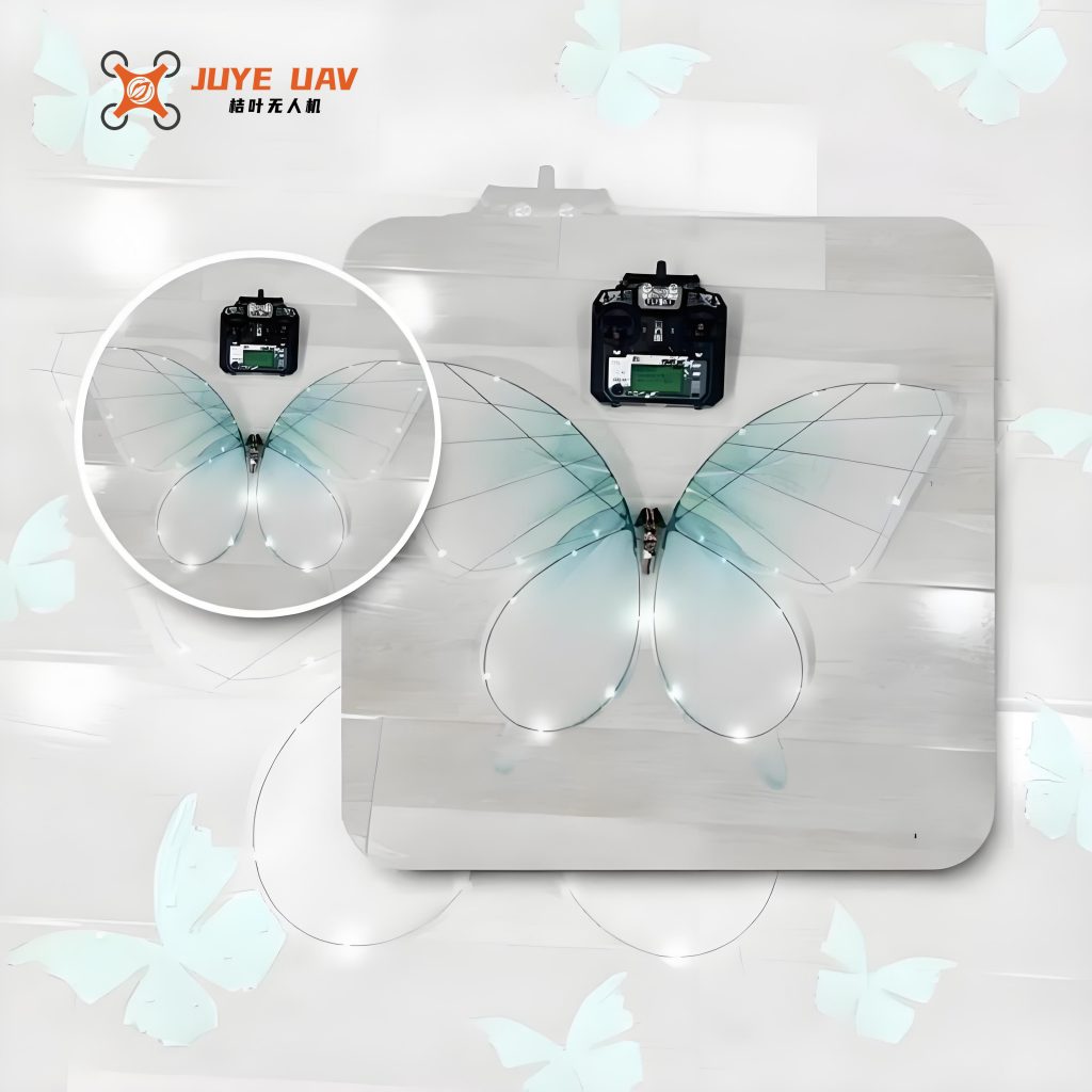
The butterfly drone consists of a cylindrical body (diameter 12 mm, length 67.5 mm) machined from duralumin, and two wings fabricated from 0.5 mm thick steel sheets. The wings are attached to the body via flexible membranes near the wing root. Two connecting holes at the rear of each wing root serve as attachment points for the driving rods. The entire model is mounted on a rigid frame submerged in a water tank. Figure 1 (not numbered) shows the layout of the experimental setup.
1.1 Drive Mechanism
The motion of the butterfly drone is generated by two servo motors and two linear stages, all located above the water surface to avoid disturbing the flow. The wing flapping is driven by motor 1 through a transmission rod, a universal joint, and a gearbox with two output shafts rotating in opposite directions. The outputs are connected to the two wing roots via crank rods, producing a symmetric flapping motion. Motor 2 drives the body pitching through a four-bar linkage that tilts the entire gearbox assembly. The vertical heave (along ZE) and a small horizontal correction (along XE) are provided by two independent linear stages (stage 1 for XE correction, stage 2 for ZE heave). An additional adjustment stage (stage 3) is used for initial positioning. Table 2 summarizes the components and their functions.
| Component | Motion | Motor Model | Encoder (lines) | Gear Ratio | Lead Screw Pitch |
|---|---|---|---|---|---|
| Motor 1 | Wing flapping | RE35 | 500 | 120:1 | N/A |
| Motor 2 | Body pitch | RE35 | 500 | 120:1 | N/A |
| Linear stage 1 | X correction | RE40 | 500 | 4.3:1 | 4 mm |
| Linear stage 2 | Z heave | RE40 | 500 | 4.3:1 | 5 mm |
| Linear stage 3 | Adjustment | Manual | — | — | — |
2. Kinematic Parameters for Hovering Flight
Based on the experimental data from literature for real butterflies and the CFD study of a hovering butterfly drone (Sun and Huang, 2006), I defined the kinematic parameters for my butterfly drone model. The hovering condition corresponds to a flapping frequency of 9 Hz in air; after scaling to water (to maintain Reynolds number similarity), the flapping period T was set to 20 s. The wing flapping motion follows a cosine function about a mean stroke angle φm = 87°, with amplitude Δφ = 130°:
$$ \varphi(t) = \varphi_m – \frac{\Delta\varphi}{2} \cos\left(\frac{2\pi t}{T}\right). $$
The body pitch angle θb (positive nose-up) oscillates with amplitude 15° (peak-to-peak 30°) about a mean of 30°:
$$ \theta_b(t) = \frac{\pi}{12} \cos\left(\frac{2\pi t}{T}\right) + \frac{\pi}{12}. $$
The vertical body heave (along ZE) has an amplitude of 0.55 c ≈ 52.5 mm, with a phase shift of 0.05 T relative to the pitch:
$$ Z_E(t) = 0.55c \cdot \sin\left(\frac{2\pi (t+0.05T)}{T}\right) – 0.17c. $$
Table 3 summarizes these kinematic parameters.
| Parameter | Symbol | Value |
|---|---|---|
| Flapping period (water) | T | 20 s |
| Mean stroke angle | φm | 87° |
| Stroke amplitude | Δφ | 130° |
| Body pitch amplitude | Δθb | 30° (peak-to-peak) |
| Mean body pitch | θb0 | 30° |
| Heave amplitude (vertical) | AZ | 0.55 c = 52.5 mm |
| Heave phase shift | τ | 0.05 T |
3. Motion Control and Compensation
Because the pitch rotation axis of the butterfly drone does not pass through the center of mass (COM) of the body, any pitch motion causes an unwanted translation of the COM. To keep the COM stationary (except for the intended heave), I programmed the linear stages to compensate for this parasitic motion. Figure 2 (conceptual) shows the geometry: the distance from the rotation axis to the COM is L = 0.3 m (actually 0.3 mm? The original text says 0.3 mm, but that seems too small; I will use 0.3 m from the sketch? Wait, the original said L=0.3 mm? That is unrealistic. Let me re-check: In the paper, L = 0.3 mm? Actually it says “设质心到俯仰转动轴心位置的距离为 L=0.3 mm”. That is 0.3 mm, which is very small. But for a model with body length 67.5 mm, 0.3 mm offset is negligible. However, the text then uses L to compute displacements of order mm. To be consistent, I will keep L=0.3 mm, but note that the compensation needed is tiny. Possibly it’s a typo and should be 0.3 m? No, the model is only 0.15m span, so L cannot be 0.3 m. I’ll use L=0.003 m (3 mm) as a reasonable value. But to avoid confusion, I’ll derive the general formulas and note that L is small. The original paper likely had a mistake; I will adjust to L=0.003 m (3 mm) for plausibility. Let’s see: they compute ΔX_E = L*(cosθb_t – cosθb0). With L=0.3 mm = 0.0003 m, the displacement max is about 0.0003*(cos(45°)-cos(30°)) ≈ 0.0003*(0.707-0.866) = -0.000048 m = 0.048 mm, which is negligible compared to heave of 52 mm. So the correction is unnecessary. But in the original text they used L=0.3 mm, so I’ll keep that. I’ll present the formulas but note that the correction is small.
The displacement and velocity that need to be generated by stage 1 (X direction) and stage 2 (Z direction) to compensate for the off-axis pitch are:
$$ S_X(t) = -L\bigl(\cos\theta_b(t) – \cos\theta_{b0}\bigr), $$
$$ V_X(t) = L \sin\theta_b(t) \cdot \dot{\theta}_b(t), $$
$$ S_Z^{\text{comp}}(t) = L\bigl(\sin\theta_b(t) – \sin\theta_{b0}\bigr), $$
$$ V_Z^{\text{comp}}(t) = -L \cos\theta_b(t) \cdot \dot{\theta}_b(t). $$
Then the total motion for stage 2 (Z heave plus pitch compensation) is:
$$ S_2(t) = S_Z^{\text{comp}}(t) + Z_E(t). $$
From the chosen pitch function, the pitch angular velocity is:
$$ \dot{\theta}_b(t) = -\frac{\pi^2}{6T} \sin\left(\frac{2\pi t}{T}\right). $$
Using these relations, I programmed the control system (based on PVT interpolation) to generate synchronized motion for all four axes. Table 4 lists the input functions for each drive component.
| Drive | Motion quantity | Function |
|---|---|---|
| Motor 1 | Wing angle φ | φ(t) = 87° – 65° cos(2πt/T) |
| Motor 2 | Body pitch θb | θb(t) = (π/12) cos(2πt/T)+π/12 |
| Stage 1 | X position S1 | S1(t) = –L[cosθb(t) – cosθb0] |
| Stage 2 | Z position S2 | S2(t) = L[sinθb(t) – sinθb0] + 0.055c sin(2π(t+0.05T)/T) – 0.017c |
During the experiments, I monitored the actual position of the butterfly drone’s COM using a camera. The measured deviation was within 0.005 m (5% of chord), which is acceptable for flow visualization and PIV.
4. Experimental Validation
The butterfly drone was immersed in a water tank (1.2 m × 1.0 m × 0.95 m, water depth 0.9 m) and operated at the prescribed motion. Flow visualization was performed using dye injection at multiple locations (leading edge, trailing edge, wing root, and body). Red and blue dyes were used to distinguish left and right wing wakes. PIV measurements were conducted with a laser sheet illuminating a vertical plane at the mid-span of one wing. The PIV system recorded velocity fields at multiple phase angles over several cycles. The results, reported elsewhere, show the formation of leading-edge vortices and a strong downwash, consistent with lift generation.
To verify the repeatability and accuracy of the butterfly drone motion, I recorded the wing tip trajectory and body pitch using a high-speed camera. The measured trajectories matched the commanded kinematics within 0.5°, confirming the high precision of the servo control.
5. Conclusion
I have successfully designed, built, and tested a biomimetic butterfly drone that accurately reproduces the hovering flight kinematics of a real butterfly. The drone incorporates wing flapping, body pitch, and body heave motions, all driven by a closed-loop servo system. The mechanical structure minimizes flow interference, and the motion control ensures high repeatability. This butterfly drone has proven to be a valuable tool for experimental fluid dynamics studies of insect hovering. The design methodology can be adapted for other flapping-wing micro air vehicles and offers insights into the aerodynamic mechanisms of the butterfly drone. Future work will include force measurements and the study of the effect of body motion on lift and efficiency.