
The rapid proliferation of unmanned aerial vehicles (UAVs), particularly those characterized as “low, slow, and small” (LSS) targets, presents a formidable challenge to modern defense and security infrastructure. These systems are difficult to detect, track, and neutralize using conventional means, thereby escalating threats in both military and civilian domains. In response, the development of directed energy weapons, especially high-energy laser (HEL) systems, has emerged as a pivotal solution for effective anti-UAV operations. This article delves into the current state-of-the-art, core technologies, and future trajectories of laser-based anti-UAV systems. From my perspective as a researcher in this field, I will synthesize key advancements, employing tables and mathematical formulations to elucidate complex concepts, and underscore the critical role of integrated, intelligent approaches in countering evolving UAV threats.
The essence of an anti-UAV laser system lies in its ability to deliver concentrated photonic energy to disable or destroy a UAV’s critical components. The operational sequence follows a detect-track-engage paradigm, which demands high precision and rapid response. The limitations of traditional kinetic solutions—such as cost-ineffectiveness against cheap drones and collateral damage risks—have accelerated the shift towards directed energy. This analysis will explore the technological pillars enabling this shift: multi-modal detection and identification, high-precision photoelectric tracking and aiming, and mechanisms of laser-induced damage. Furthermore, I will project future developments centered on intelligent, networked anti-UAV architectures capable of defeating coordinated swarm attacks.
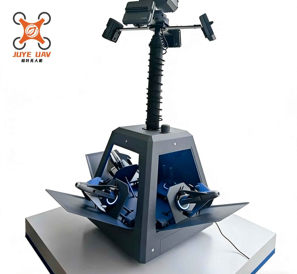
The global landscape for anti-UAV laser development is highly competitive. Several nations have demonstrated operational prototypes, signaling a transition from laboratory research to field deployment. The United States has been a frontrunner, with programs like the High Energy Laser Mobile Demonstrator (HELMD) and the Laser Weapon System (LaWS) achieving milestones in shooting down drones at ranges of several kilometers. These systems, often mounted on mobile ground vehicles or naval vessels, showcase the increasing maturity of solid-state laser technology at power levels from 10 kW to over 100 kW. European initiatives, such as Germany’s Rheinmetall “Skyguard” system, utilize beam combining techniques to aggregate power from multiple laser modules, demonstrating effective engagement in diverse weather conditions. Meanwhile, other military powers are advancing their own counter-UAV architectures, integrating laser weapons into layered defense networks. The overarching trend is toward more compact, efficient, and powerful laser sources that can be deployed across multiple platforms—land, sea, air, and potentially space—to create a seamless anti-UAV umbrella.
The effectiveness of any anti-UAV system is fundamentally constrained by its ability to first find and classify the threat. LSS drones exhibit radar cross-sections (RCS) comparable to birds, fly at low altitudes within ground clutter, and can hover or move erratically, confounding conventional sensors. Therefore, a synergistic fusion of disparate detection modalities is essential. The primary technologies can be summarized and compared as follows:
| Sensing Modality | Core Principle & Advantages | Key Limitations for Anti-UAV | Typical Performance Metrics |
|---|---|---|---|
| Radar Detection | Active emission of RF waves; measures time delay and Doppler shift for range, velocity, and angle. Long-range capability, all-weather operation. | Susceptible to clutter at low altitudes; difficulty distinguishing drones from birds; limited performance against slow or hovering targets; active emission compromises stealth. | Detection Range: 5-10 km for small UAVs. Angular Accuracy: ~1-5 mrad. RCS of typical mini-UAV: 0.01 – 0.1 m². |
| Radio Frequency (RF) Sensing | Passive interception of communication links between drone and controller. Provides identification of drone type and potential operator location. | Ineffective against autonomous/pre-programmed drones; congested spectral environments cause interference; limited range determined by link budget. | Detection Range: 1-5 km (dependent on transmitter power). Identification success rate: >80% in clear spectrum. |
| Electro-Optic/Infrared (EO/IR) | Passive imaging in visible and infrared bands. Provides high-resolution imagery for positive identification and precision tracking. | Performance degrades with weather (fog, rain); requires cueing from other sensors for wide-area search; can be confused by other small airborne objects. | Identification Range (Visual): 1-3 km. Thermal Detection Range: 1-2 km. Field of View: Narrow for tracking (<5°). |
| Acoustic Sensing | Passive detection of acoustic signatures from UAV motors and propellers. Low cost and good for very short-range, covert detection. | Very short effective range (<1 km); highly susceptible to ambient noise; poor directional accuracy. | Detection Range: 100-500 m. Classification accuracy: ~70-90% for distinct motor types. |
Information fusion from these sensors is a non-trivial challenge. It involves spatial and temporal registration of data, followed by algorithm-driven decision-making. A common mathematical framework for target state estimation in tracking is the Kalman Filter. For a target with state vector $\mathbf{x}_k$ (containing position, velocity) at time $k$, the filter predicts and updates based on measurements $\mathbf{z}_k$:
$$\hat{\mathbf{x}}_{k|k-1} = \mathbf{F}_k \hat{\mathbf{x}}_{k-1|k-1}$$
$$\mathbf{P}_{k|k-1} = \mathbf{F}_k \mathbf{P}_{k-1|k-1} \mathbf{F}_k^T + \mathbf{Q}_k$$
$$\mathbf{K}_k = \mathbf{P}_{k|k-1} \mathbf{H}_k^T (\mathbf{H}_k \mathbf{P}_{k|k-1} \mathbf{H}_k^T + \mathbf{R}_k)^{-1}$$
$$\hat{\mathbf{x}}_{k|k} = \hat{\mathbf{x}}_{k|k-1} + \mathbf{K}_k (\mathbf{z}_k – \mathbf{H}_k \hat{\mathbf{x}}_{k|k-1})$$
$$\mathbf{P}_{k|k} = (I – \mathbf{K}_k \mathbf{H}_k) \mathbf{P}_{k|k-1}$$
where $\mathbf{F}_k$ is the state transition model, $\mathbf{H}_k$ is the observation model, $\mathbf{Q}_k$ and $\mathbf{R}_k$ are process and measurement noise covariances, and $\mathbf{K}_k$ is the Kalman gain. For anti-UAV applications, extended or unscented Kalman filters are often used to handle non-linear dynamics.
A critical sub-problem in anti-UAV detection is distinguishing drones from birds, a task where micro-Doppler radar signatures are invaluable. The micro-Doppler effect arises from periodic movements like rotor blade rotations. The radar return signal $s(t)$ from a target with micro-motions can be modeled as:
$$s(t) = A \exp\left[j2\pi f_c t + j\frac{4\pi}{\lambda} R(t) + j\phi_m(t)\right]$$
where $A$ is amplitude, $f_c$ is carrier frequency, $\lambda$ is wavelength, $R(t)$ is the main body range, and $\phi_m(t)$ is the phase modulation due to micro-motions. For a rotor blade of length $L$ rotating at angular velocity $\Omega$, the micro-Doppler frequency $f_{mD}$ induced at a specific aspect angle is approximately:
$$f_{mD}(t) \approx \frac{2\Omega L}{\lambda} \cos(\beta) \cos(\Omega t)$$
where $\beta$ is the elevation angle of the blade. The time-frequency representation (e.g., using Short-Time Fourier Transform) of this signal reveals distinct patterns for drones versus birds, enabling feature-based classification. Deep learning models, particularly Convolutional Neural Networks (CNNs), are now being trained on such time-frequency images to achieve high discrimination accuracy, a key step in reliable anti-UAV warning systems.
Once a UAV is detected and identified, the system must achieve and maintain precise aimpoint control on a potentially maneuvering target. This is the domain of photoelectric tracking and aiming (ETA) systems. The primary challenge is to compensate for platform vibration, atmospheric turbulence, and target motion to keep the high-energy laser beam focused on a small spot on the UAV. Most advanced anti-UAV laser systems employ a dual-stage, or compound-axis, servo control architecture. The coarse tracking stage uses a gimbal-mounted system with wide field-of-view sensors (e.g., IR cameras or coarse acquisition cameras) to initially capture and follow the target over a large angular range. The fine tracking stage uses a Fast Steering Mirror (FSM) with a narrow field-of-view, high-bandwidth sensor to correct for residual errors. The control block diagram for such a system can be represented as a multi-loop feedback problem.
The performance of the coarse stage is limited by mechanical resonances and servo bandwidth. Its transfer function $G_c(s)$ often includes resonances that must be compensated:
$$G_c(s) = K_c \frac{\omega_{n_c}^2}{s^2 + 2\zeta_{c}\omega_{n_c}s + \omega_{n_c}^2} e^{-\tau_c s}$$
where $\omega_{n_c}$ is the natural frequency, $\zeta_c$ is the damping ratio, and $\tau_c$ is a delay. The fine tracking stage, typically an FSM, has a much higher bandwidth. Its response $G_f(s)$ can be modeled as:
$$G_f(s) = K_f \frac{\omega_{n_f}^2}{s^2 + 2\zeta_{f}\omega_{n_f}s + \omega_{n_f}^2}$$
where $\omega_{n_f} \gg \omega_{n_c}$. The overall pointing error $\theta_e$ is the difference between the target angle $\theta_t$ and the combined pointing angle of the gimbal $\theta_g$ and the FSM $\theta_f$: $\theta_e = \theta_t – (\theta_g + \theta_f)$. The control laws for both loops are designed to minimize this error. A common approach uses a Proportional-Integral-Derivative (PID) controller for the coarse loop and a higher-order compensator (like a lead-lag or $H_\infty$ controller) for the fine loop. The resulting pointing stability can achieve values in the microradian range, which is crucial for maintaining the lethal power density on target over the required dwell time. The alignment and calibration between the tracking sensors and the laser beam itself are also critical, described by boresight error matrices that must be dynamically corrected.
The culmination of the anti-UAV engagement is the laser-target interaction, leading to structural or functional damage. The primary kill mechanisms for laser weapons against UAVs are thermal and thermo-mechanical. The core parameter is the irradiance $I$ (power per unit area) on the target:
$$I = \frac{P}{A_{spot}} = \frac{P}{\pi (r_{spot})^2}$$
where $P$ is the laser power at the target (after atmospheric attenuation) and $r_{spot}$ is the beam radius at the target range $R$, which for a diffraction-limited beam is approximately $r_{spot} \approx \frac{\lambda R}{D}$, with $D$ being the transmitter aperture diameter. However, atmospheric turbulence causes beam wander and spreading, reducing effective irradiance. The Strehl ratio $S$ is a metric for this degradation: $S = \frac{I_{actual}}{I_{diffraction-limited}}$.
The thermal effect is governed by the heat conduction equation. For a simple model of a composite material (like a carbon-fiber UAV skin) exposed to a laser beam, the surface temperature rise $\Delta T$ can be estimated by considering one-dimensional heat flow:
$$\rho c_p \frac{\partial T}{\partial t} = k \frac{\partial^2 T}{\partial z^2} + \alpha I(t) – h(T – T_\infty) – \epsilon \sigma (T^4 – T_\infty^4)$$
where $\rho$ is density, $c_p$ is specific heat, $k$ is thermal conductivity, $\alpha$ is absorptivity at the laser wavelength, $h$ is convective heat transfer coefficient, $\epsilon$ is emissivity, $\sigma$ is Stefan-Boltzmann constant, and $T_\infty$ is ambient temperature. Ignoring radiation and convection for a short pulse, the time $t_{th}$ to reach a critical temperature $T_{crit}$ (e.g., melting point) at the surface is roughly:
$$t_{th} \approx \frac{\rho c_p (T_{crit} – T_\infty)}{\alpha I}$$
For structural failure, the laser must deliver a fluence $F$ (energy per unit area, $F = I \cdot t_{dwell}$) that exceeds a damage threshold $F_{th}$. Different materials have vastly different thresholds, as summarized below:
| UAV Component Material | Typical Laser Damage Threshold (Fluence for penetration) | Primary Damage Mechanism |
|---|---|---|
| Polymer/Carbon Fiber Composite (Skin) | 1 – 10 kJ/m² for 1 µm wavelength (continuous wave or long pulse) | Ablation, delamination, loss of structural integrity. |
| Aluminum Alloy (Frame, Motor Housing) | 10 – 100 kJ/m² for 1 µm wavelength | Melting, vaporization, hole drilling. |
| Silicon-based Imaging Sensor (EO Payload) | 0.1 – 1 kJ/m² | Thermal runaway, blinding/dazzling (soft kill). |
| Polycarbonate (Propeller) | 0.5 – 5 kJ/m² | Melting, deformation leading to imbalance. |
The required dwell time $t_{dwell}$ for a given laser power $P$, target range $R$, and material threshold $F_{th}$ is:
$$t_{dwell} \geq \frac{F_{th} \cdot A_{spot}}{P \cdot S \cdot T_{atm}}$$
where $T_{atm}$ is the atmospheric transmission factor (from Beer-Lambert law: $T_{atm} = e^{-\beta R}$, with $\beta$ as the attenuation coefficient) and $S$ is the Strehl ratio. This equation highlights the trade-offs in anti-UAV laser design: higher power reduces dwell time, but larger apertures and adaptive optics are needed to maintain a small spot size and compensate for turbulence.
In the context of drone swarms, the problem escalates to dynamic weapon-target assignment (WTA). With multiple incoming UAVs and potentially multiple laser assets, an optimal engagement schedule must be computed. This is a constrained optimization problem. Let $n$ be the number of threats and $m$ the number of laser assets. Define a binary decision variable $x_{ij} = 1$ if laser $i$ is assigned to engage threat $j$, and 0 otherwise. Let $p_{ij}$ be the probability of kill (Pk) if laser $i$ engages threat $j$, which is a function of the dwell time, laser power, and target vulnerability. A common objective is to maximize the total expected threat value neutralized:
$$\text{Maximize } Z = \sum_{j=1}^{n} v_j \left(1 – \prod_{i=1}^{m} (1 – p_{ij})^{x_{ij}}\right)$$
subject to constraints such as:
$$\sum_{j=1}^{n} x_{ij} \leq 1 \quad \forall i \text{ (each laser engages at most one target at a time)}$$
$$\sum_{i=1}^{m} x_{ij} \leq 1 \quad \forall j \text{ (each target assigned to at most one laser, or relaxed for salvo)}$$
and timing constraints that account for the dwell time $t_{dwell, ij}$ and slew time between targets. This integer programming problem is NP-hard for large $n$ and $m$, necessitating heuristic or metaheuristic solutions like Genetic Algorithms (GA), Particle Swarm Optimization (PSO), or Ant Colony Optimization (ACO). For real-time anti-UAV defense, these algorithms must be highly efficient. The fitness function in a GA for WTA could incorporate not just Pk but also the time-to-intercept and threat priority weights $w_j$:
$$Fitness = \sum_{j} w_j \cdot p_{ij} \cdot \exp(-\gamma \cdot t_{engage,j})$$
where $\gamma$ is a discount factor favoring earlier engagements.
Beyond engagement, Battle Damage Assessment (BDA) is crucial for determining re-engagement necessity. For laser anti-UAV systems, BDA can involve monitoring the target’s kinematic behavior (e.g., loss of control, deceleration, change in trajectory) via tracking sensors, or analyzing spectroscopic signatures of plume emissions if material vaporization occurs. Machine learning classifiers trained on post-engagement sensor data (RF signal loss, visual/IR image degradation) are being developed to provide real-time BDA estimates.
Looking forward, the evolution of anti-UAV laser systems will be shaped by several converging trends. First, the integration of Artificial Intelligence (AI) and Machine Learning (ML) will permeate every layer, from detection to decision-making. Deep neural networks will enable robust classification of UAVs in cluttered environments, even from fused sensor snippets. Reinforcement learning agents could manage the dynamic WTA problem, adapting to novel swarm tactics in real-time. Secondly, laser technology itself will advance toward more efficient, compact, and higher-power sources. Fiber laser combiners and spectral beam combining are pushing powers into the 300-500 kW regime while improving electrical-to-optical efficiency. These developments will enable the deployment of effective anti-UAV systems on smaller platforms, including tactical vehicles and unmanned ground or aerial systems themselves. Thirdly, the concept of “system-of-systems” or networked cooperative engagement will become paramount. A future anti-UAV network might consist of distributed low-power laser dazzlers, high-power killer lasers, drone-based interceptor platforms, and electronic warfare jammers, all orchestrated by a central or distributed AI command. The kill chain will be compressed through predictive cueing and automated engagement protocols.
Finally, countering autonomous drone swarms represents the ultimate challenge. Swarm intelligence introduces emergent behaviors that are difficult to predict. Future anti-UAV systems will need to employ counter-swarm tactics, potentially using swarms of defensive drones equipped with lasers or nets, or deploying wide-area pulsed lasers with a lower fluence per drone but capable of affecting multiple targets simultaneously. The mathematical modeling of such swarm-on-swarm engagements will involve complex agent-based simulations and game theory. The payoff function in a differential game between an attacker swarm $A$ and a defender laser system $D$ could be formulated to minimize the number of attackers reaching a protected asset, considering energy and time constraints for the defender.
In conclusion, the field of laser-based anti-UAV defense is rapidly transitioning from technological demonstration to operational deployment. The core technical hurdles—efficient multi-sensor fusion, ultra-precise tracking, efficient high-power lasers, and intelligent resource allocation—are being addressed through interdisciplinary advances in photonics, control theory, materials science, and artificial intelligence. The future of air defense against asymmetric UAV threats will undoubtedly rely heavily on directed energy systems. However, their true potential will only be realized when they are embedded within a holistic, adaptive, and intelligent network capable of perceiving, deciding, and acting at the speed of light. As the threat evolves, so too must our countermeasures, driving continuous innovation in the science and engineering of anti-UAV systems.