
In this study, I investigate the aerodynamic modeling and path optimization challenges associated with the wing docking process of fixed-wing drones. The aerial docking problem has long been a critical bottleneck restricting the development of chained-wing drone technology. To address this, I develop a comprehensive aerodynamic model using the numerical lifting-line method and propose a path planning approach based on the Dijkstra algorithm. Through systematic simulation and analysis, I demonstrate that the optimized docking path can significantly reduce wingtip vortex interference during the docking maneuver.
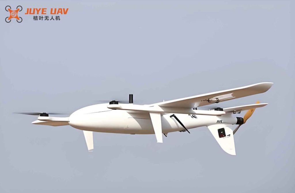
Table 1 summarizes the key parameters of the fixed-wing drone used throughout my study.
| Parameter | Value |
|---|---|
| Airfoil | NACA0010 |
| Weight | 20 N |
| Half span | 2 m |
| Chord length | 1 m |
| Fuselage length | 1 m |
| Chord length of vertical tail | 0.4 m |
| Span length of vertical tail | 0.5 m |
| Sweep of vertical tail | 20° |
| Chord length of horizontal tail | 0.4 m |
| Span length of horizontal tail | 0.5 m |
| Sweep of horizontal tail | 20° |
1. Introduction
The fixed-wing drone has emerged as a versatile platform for various civilian and military applications. However, individual fixed-wing drones often suffer from limitations such as单一 functionality, poor versatility, short endurance, and weak survivability. To overcome these drawbacks, a novel concept known as the chained-wing drone, based on wingtip docking, has gained increasing research attention. The chained-wing aircraft concept was originally proposed by the German scientist Richard Vogt, who envisioned extending fighter range by attaching “free-floating” flight modules at the wingtips that also carry fuel. Due to the increased aspect ratio from these modules, induced drag is effectively reduced.
Historical flight tests, such as the Q-14 and C-47 wing docking experiment conducted by the U.S. Air Force in 1949, and the subsequent Tip-Tow project involving B-29 bombers and F-84 jets, have demonstrated that wingtip vortices create complex aerodynamic interference during the docking process. These tests placed extremely high demands on piloting skills. With the advancement of drone measurement and control software and hardware technologies, the chained-wing drone concept has regained vitality, offering significant advantages in aerodynamic performance improvement, range extension, and success rate enhancement for complex missions.
For a fixed-wing drone, the aerial docking maneuver requires precise control and reliable aerodynamic modeling. The aerodynamic coupling effects between two closely flying fixed-wing drones are intense and highly nonlinear. Therefore, developing an accurate yet computationally efficient aerodynamic model for the wing docking process is essential for the design of flight control systems and path planning algorithms.
2. Aerodynamic Modeling Methodology
In my research, I adopt the G-H numerical lifting-line method to model the aerodynamic forces during the wing docking process of fixed-wing drones. This method represents a significant advancement over traditional lifting-line theories, as it eliminates singularity issues and can handle complex three-dimensional wing geometries.
2.1 Fundamental Principles of the G-H Method
The lifting-line theory was originally proposed by Prandtl for aerodynamic modeling of wings. Traditional lifting-line methods suffer from singularities when the curvature at the control points is non-zero or when the lifting line is not perpendicular to the freestream velocity direction. Phillips and Snyder developed a numerical approach to Prandtl’s lifting-line theory, but the singularity problem persisted. Reid and Hunsaker then developed the R-H method, which introduced the concept of the effective locus of aerodynamic center (LAC) to replace the original lifting line, ensuring zero curvature at control points.
Building upon the R-H method, Goates and Hunsaker extended the approach to create the G-H method, which can handle arbitrary numbers of wings with fully three-dimensional geometries. In the G-H method, the attachment portions of the vortex system and the control points are placed on the quarter-chord line.
2.2 Geometric Definitions
I first introduce the dimensionless quantity s, representing the displacement from the wing root along the lifting line projected onto the y-z plane of the fuselage, normalized by the half-span of the wing. The value of s is negative on the left half of the wing and positive on the right half. In the G-H method, the sweep angle Λ is defined as positive when the quarter-chord line rotates around the z-axis according to the right-hand rule. The dihedral angle Γ is defined as positive when the wing rotates around the x-axis according to the right-hand rule.
The original lifting line position function rLL(s) in the G-H method is expressed as:
$$ \mathbf{r}_{LL}(s) = \mathbf{r}_{LL}(0) + \frac{b}{2} \begin{bmatrix} -\int_0^s \tan\Lambda(s) \, ds \\ \int_0^s \cos\Gamma(s) \, ds \\ \int_0^s \sin\Gamma(s) \, ds \end{bmatrix}, \quad -1 \leq s \leq 1 $$
where Λ(s) and Γ(s) are the local sweep angle and local dihedral angle, respectively, b/2 is the half-span, and rLL(0) is the known position of the quarter-chord line at the wing root.
To improve convergence, I use a cosine distribution for the N control points on the right half-wing:
$$ s_i = \frac{1}{2} \left[ 1 – \cos\left( \frac{\pi}{2N} + \frac{i\pi}{N} \right) \right], \quad i = 0, 1, \ldots, N-1 $$
For the control points on the left half-wing, I simply take the negative of the corresponding si values.
To ensure zero curvature at the control points, the effective lifting line position at control point i is defined as:
$$ \tilde{\mathbf{r}}^i_{LL}(s) = (1 – e^{-\sigma(s-s_i)^2}) \mathbf{r}_{LL}(s) + e^{-\sigma(s-s_i)^2} \left[ \mathbf{r}_{LL}(s_i) + \left. \frac{d\mathbf{r}_{LL}}{ds} \right|_{s=s_i} (s-s_i) \right] $$
where σ is a positive real number related to the dimensionless distance Δs. When s ≥ Δs, the straightness of the effective lifting line is below 0.018%. The relationship between σ and Δsb is given by:
$$ \sigma = \frac{2}{(\Delta s_b \cos\Lambda)^2} $$
where Δsb is called the coordination distance. In my simulations, this dimensionless parameter is set to 1.
2.3 Definition of Direction Vectors and Trailing Vortices
To calculate the sectional angle of attack and define the trailing vortices, I define unit axial, normal, and spanwise vectors at each vortex node and control point. The axial vector ua points backward along the chord of the local airfoil section, the normal vector un points downward perpendicular to the local airfoil section plane, and the spanwise vector us points toward the right wingtip. These vectors are expressed as:
$$ \mathbf{u}_s = [0, \cos\Gamma, \sin\Gamma]^T $$
$$ \mathbf{u}_a = [-\cos\tau, -\sin\tau\sin\Gamma, \sin\tau\cos\Gamma]^T $$
$$ \mathbf{u}_n = [-\sin\tau, \cos\tau\sin\Gamma, -\cos\tau\cos\Gamma]^T $$
where τ is the local twist angle, considered positive when rotating around us according to the right-hand rule.
Step changes in dihedral angle Γ and twist angle τ can cause discontinuities in the axial unit vector, affecting the accuracy of the numerical solution. To eliminate these discontinuities, I use a function of s:
$$ \tilde{\mathbf{u}}_{a\Lambda}(s) = (1 – e^{-\sigma(s-s_i)^2}) \mathbf{u}_{a\Lambda}(s) + e^{-\sigma(s-s_i)^2} \mathbf{u}_{a\Lambda}(s_i) $$
The position of each vortex node is then defined as:
$$ \mathbf{r}_{joint,i} = \mathbf{r}_{LL}(s_i) + \delta c_i \tilde{\mathbf{u}}_{a\Lambda}(s_i) $$
Starting from the vortex nodes, the trailing vortex segments extend infinitely along the local velocity direction. The expression for the trailing vortex segment is:
$$ \mathbf{u}_{trailing,i} = \frac{\mathbf{u}_\infty – \boldsymbol{\omega} \times (\mathbf{r}_{joint,i} – \mathbf{r}_{cg})}{\|\mathbf{u}_\infty – \boldsymbol{\omega} \times (\mathbf{r}_{joint,i} – \mathbf{r}_{cg})\|} $$
where ω is the angular velocity vector in the body coordinate system, and rcg is the center of gravity position in the body coordinate system.
2.4 Aerodynamic Forces on Swept Segments
In the G-H method, the cross-section of the wing perpendicular to the lifting line is used as the airfoil section. This leads to the concepts of effective section geometry, effective velocity, and effective angle of attack. The chord length of the effective section, called the swept chord length, is:
$$ c_\Lambda = c \cos\Lambda $$
where Λ is the local sweep angle.
Since the effective airfoil section plane is perpendicular to the lifting line, I only need to consider the resultant velocity in that plane. The effective velocity is:
$$ \mathbf{V}_\Lambda = \mathbf{P}_{eff} \cdot \mathbf{V} $$
where Peff = I – usΛusΛT, and I is the identity matrix.
Based on the effective velocity, the effective angle of attack is defined as:
$$ \alpha_\Lambda = \arctan\left( \frac{\mathbf{V}_\Lambda \cdot \mathbf{u}_{n\Lambda}}{\mathbf{V}_\Lambda \cdot \mathbf{u}_{a\Lambda}} \right) $$
To account for viscous effects in the numerical lifting-line method, I compute the effective Reynolds number based on the effective section geometry and effective velocity:
$$ Re_\Lambda = \frac{\|\mathbf{V}_\Lambda\| c_\Lambda}{\nu} $$
where ν is the kinematic viscosity. The effective Reynolds number and effective angle of attack are used to determine the viscous lift and moment coefficients.
Using thin airfoil theory, the zero-lift angle of attack for a swept section is:
$$ \alpha_{L0\Lambda} = \frac{\alpha_{L0}}{\cos\Lambda} $$
This relationship indicates that the sweep angle affects the aerodynamic characteristics of the airfoil section solely through the change in the zero-lift angle of attack. For a swept wing and its corresponding unswept wing, the lift curve of the former is simply a horizontal translation of the lift curve of the latter.
Based on this relationship, I approximate:
$$ \tilde{C}_{L\Lambda}(\alpha_\Lambda) \approx \tilde{C}_L(\alpha_\Lambda + \alpha_{L0} – \alpha_{L0\Lambda}) $$
Performing a Taylor expansion of CLΛ with respect to αΛ at αL0 – αL0Λ and neglecting higher-order terms, I obtain:
$$ \tilde{C}_{L\Lambda}(\alpha_\Lambda) \approx \tilde{C}_{L\Lambda}(\alpha_\Lambda) + \tilde{C}_{L,\alpha}(\alpha_{L0} – \alpha_{L0\Lambda}) $$
This approximation has high accuracy in the linear range of the lift curve and when αL0 – αL0Λ is small.
Similar to the zero-lift angle of attack calculation, the moment coefficient about the quarter-chord line from thin airfoil theory is:
$$ \tilde{C}_{mc/4\Lambda} = \frac{\tilde{C}_{mc/4}}{\cos\Lambda} $$
where C̃mc/4 is the moment coefficient of the unswept wing segment.
To calculate the aerodynamic force on a discrete swept wing segment, I first compute the segment area:
$$ \Delta S_i = \frac{b}{4} (s_{i+1} – s_i)(c_{i+1} + c_i) $$
Based on the effective section velocity and the sectional lift coefficient, the lift of this discrete wing segment is:
$$ \Delta L_i = \frac{1}{2} \rho \|\mathbf{V}_{\Lambda,i}\|^2 \tilde{C}_{L\Lambda,i} \Delta S_i $$
The moment about the quarter-chord line is:
$$ \Delta M_i = \frac{1}{2} \rho \|\mathbf{V}_{\Lambda,i}\|^2 \tilde{C}_{L\Lambda,i} c_{\Lambda i} \Delta S_i $$
For the drag coefficient calculation, I assume that swept and unswept wings have the same drag coefficient at low angles of attack:
$$ \Delta D_i = \frac{1}{2} \rho \| \mathbf{V}_i \| \mathbf{V}_i \tilde{C}_{D,i} \Delta S_i $$
where C̃D,i is the drag coefficient of the corresponding unswept wing segment computed based on the effective Reynolds number and effective angle of attack.
2.5 Governing Equations and Solution Procedure
Using the P-S method to compute the induced velocity, the governing equation of the G-H method at control point i is:
$$ 2 \| \mathbf{V}_{\Lambda,i} \times d\mathbf{l}_i \| \Gamma_i – \|\mathbf{V}_{\Lambda,i}\|^2 \tilde{C}_{L\Lambda,i} \Delta S_i = 0 $$
where VΛ,i is the effective velocity at control point i, dli = rLL(si+1) – rLL(si), and Γi is the vortex strength.
Under the assumptions of small angles of attack, sideslip angles, twist angles, and rotational speeds much smaller than the freestream velocity, the angle of attack can be approximated as:
$$ \alpha_{\Lambda,i} = \frac{1}{V_{\infty\Lambda,i}} \left[ (\mathbf{V}_{\infty,i} – \boldsymbol{\omega} \times \mathbf{r}_i) \cdot \mathbf{u}_{n\Lambda,i} + \left( \sum_{j=1}^N \Gamma_{ij} \mathbf{v}_{ji} \right) \cdot \mathbf{u}_{n\Lambda,i} \right] $$
Using a linear approximation for the lift coefficient of the swept wing segment:
$$ \tilde{C}_{L\Lambda,i} \approx \tilde{C}_{L,\alpha_i} (\alpha_{\Lambda,i} – \alpha_{L0\Lambda,i}) $$
and assuming VΛ,i ≈ V∞, the governing equation can be linearized as:
$$ 2 \| \mathbf{V}_{\infty+\omega\Lambda,i} \times d\mathbf{l}_i \| \Gamma_i – V_{\infty\Lambda,i} \tilde{C}_{L,\alpha_i} \Delta S_i \left( \sum_{j=1}^N \Gamma_j \mathbf{v}_{ji} \right) \cdot \mathbf{u}_{n\Lambda,i} = V_{\infty\Lambda,i}^2 \tilde{C}_{L,\alpha_i} \Delta S_i \left[ \frac{1}{V_\infty} (\mathbf{V}_{\infty+\omega\Lambda,i} \cdot \mathbf{u}_{n\Lambda,i}) – \alpha_{L0\Lambda,i} \right] $$
For nonlinear cases, I use Newton iteration to solve the system. Writing the vortex strengths as a vector Γ, the governing equation can be expressed in vector form as:
$$ \mathbf{f}(\boldsymbol{\Gamma}) = \mathbf{R} $$
where fi(Γ) = 2\|VΛ,i × dli\|Γi – ‖VΛ,i‖²C̃LΛ,iΔSi, and R is the residual vector. The Newton correction formula is:
$$ \mathbf{J} \Delta\boldsymbol{\Gamma} = -\mathbf{R} $$
where J is the Jacobian matrix of f(Γ). After determining ΔΓ, the vortex strengths are updated iteratively:
$$ \boldsymbol{\Gamma}^{k+1} = \boldsymbol{\Gamma}^k + \psi \Delta\boldsymbol{\Gamma} $$
where k is the iteration step and ψ is the relaxation factor. Once the vortex strengths are obtained, the inviscid force on each attached vortex segment is:
$$ \Delta\mathbf{F}_{\Gamma,i} = \rho \Gamma_i \mathbf{V}_{\Lambda,i} \times d\mathbf{l}_i $$
The total force on each wing segment, including both viscous and inviscid contributions, is:
$$ \mathbf{F}_{total} = \sum_{i=1}^N (\Delta\mathbf{D}_i + \Delta\mathbf{F}_{\Gamma,i}) $$
According to the definitions in the G-H method, the lift, drag, and side forces are:
$$ L = \mathbf{F}_{total} \cdot \frac{\hat{\mathbf{u}}_\infty \times \hat{\mathbf{i}}_y}{\|\hat{\mathbf{u}}_\infty \times \hat{\mathbf{i}}_y\|} $$
$$ D = \mathbf{F}_{total} \cdot \hat{\mathbf{u}}_\infty $$
$$ S = \mathbf{F}_{total} – D\hat{\mathbf{u}}_\infty – L\hat{\mathbf{u}}_L $$
The moment about the center of gravity for each discrete wing segment is:
$$ \Delta\mathbf{M}_i = (\mathbf{r}_{LL,i} – \mathbf{r}_{CG}) \times (\Delta\mathbf{F}_{\Gamma,i} + \Delta\mathbf{D}_i) + \frac{1}{2} \rho_i \|\mathbf{V}_{\Lambda,i}\|^2 \tilde{C}_{m\Lambda,i} \Delta S_i c_{\Lambda i} \mathbf{u}_{s\Lambda,i} $$
The total moment acting on the fixed-wing drone is:
$$ \mathbf{M} = \sum_{j=1}^N \Delta\mathbf{M}_i $$
To validate the G-H numerical lifting-line method, I computed the lift coefficients of a swept wing with a 45° sweep angle using the NACA0010 airfoil at different angles of attack. The results showed excellent agreement with reference data, confirming the reliability of this method for aerodynamic modeling of fixed-wing drones.
3. Aerodynamic Database Generation
Using the G-H method, I generated a comprehensive aerodynamic database for the wing docking process of fixed-wing drones. The simulation parameters are summarized in Table 2.
| Parameter | Value |
|---|---|
| Velocity | 10 m/s |
| Angle of attack | 2° |
| Spanwise gap range | 0, 0.4, 0.8, …, 3.6, 4.0 m |
| Chordwise gap range | 0, 0.4, 0.8, …, 3.6, 4.0 m |
I simplified the wing docking problem to the scenario where two fixed-wing drones are on the same horizontal plane performing wingtip docking. The leading fixed-wing drone, positioned at the left front, maintains steady straight-and-level flight. The following fixed-wing drone, positioned at the right rear, gradually approaches on the same horizontal plane, with both drones maintaining the same angle of attack.
Using the origin at the state when the two fixed-wing drones have completed docking, I established a planar Cartesian coordinate system. I selected different position points in both the spanwise and chordwise directions to compute the aerodynamic characteristics at various relative positions during the wing docking process.
From the aerodynamic database, I observed significant aerodynamic coupling effects during the wingtip docking process. Table 3 presents the lift and rolling moment data for the following fixed-wing drone at selected relative positions.
| Spanwise gap (m) | Chordwise gap (m) | Lift (N) | Rolling moment (N·m) |
|---|---|---|---|
| 0.0 | 0.0 | 18.24 | 0.852 |
| 0.4 | 0.0 | 17.86 | 0.734 |
| 0.8 | 0.0 | 17.41 | 0.612 |
| 1.2 | 0.0 | 17.03 | 0.498 |
| 1.6 | 0.0 | 16.72 | 0.387 |
| 2.0 | 0.0 | 16.48 | 0.285 |
| 2.4 | 0.0 | 16.31 | 0.194 |
| 2.8 | 0.0 | 16.19 | 0.118 |
| 3.2 | 0.0 | 16.11 | 0.062 |
| 3.6 | 0.0 | 16.06 | 0.028 |
| 4.0 | 0.0 | 16.03 | 0.011 |
Table 4 shows the aerodynamic data when varying the chordwise gap while keeping the spanwise gap at zero.
| Chordwise gap (m) | Lift (N) | Rolling moment (N·m) |
|---|---|---|
| 0.0 | 18.24 | 0.852 |
| 0.4 | 18.08 | 0.801 |
| 0.8 | 17.85 | 0.723 |
| 1.2 | 17.56 | 0.634 |
| 1.6 | 17.28 | 0.542 |
| 2.0 | 17.01 | 0.448 |
| 2.4 | 16.78 | 0.356 |
| 2.8 | 16.58 | 0.268 |
| 3.2 | 16.42 | 0.189 |
| 3.6 | 16.29 | 0.118 |
| 4.0 | 16.19 | 0.062 |
From these results, I observed that the aerodynamic coupling effects intensify as the distance between the two fixed-wing drones decreases. The lift and rolling moment on the following fixed-wing drone show significant variations when the two drones are in close proximity. Specifically, when the spanwise gap is small, the lift increases substantially due to the upwash effect from the leading fixed-wing drone’s wingtip vortex. Meanwhile, the rolling moment also increases significantly, which could pose control challenges during the docking maneuver.
Table 5 presents the full aerodynamic database mapping for the following fixed-wing drone across the entire relative position space.
| Spanwise gap (m) | Chordwise gap (m) | Lift (N) | Drag (N) | Rolling moment (N·m) | Pitching moment (N·m) |
|---|---|---|---|---|---|
| 0.0 | 0.0 | 18.24 | 1.82 | 0.852 | 0.124 |
| 0.0 | 1.0 | 17.42 | 1.68 | 0.684 | 0.098 |
| 0.0 | 2.0 | 17.01 | 1.62 | 0.448 | 0.072 |
| 0.0 | 3.0 | 16.58 | 1.58 | 0.268 | 0.045 |
| 0.0 | 4.0 | 16.19 | 1.55 | 0.062 | 0.018 |
| 1.0 | 0.0 | 17.25 | 1.71 | 0.548 | 0.086 |
| 1.0 | 1.0 | 16.88 | 1.64 | 0.412 | 0.064 |
| 1.0 | 2.0 | 16.52 | 1.59 | 0.298 | 0.048 |
| 1.0 | 3.0 | 16.24 | 1.56 | 0.152 | 0.032 |
| 1.0 | 4.0 | 16.08 | 1.54 | 0.048 | 0.014 |
| 2.0 | 0.0 | 16.48 | 1.63 | 0.285 | 0.052 |
| 2.0 | 1.0 | 16.31 | 1.60 | 0.194 | 0.038 |
| 2.0 | 2.0 | 16.18 | 1.57 | 0.118 | 0.026 |
| 2.0 | 3.0 | 16.08 | 1.55 | 0.062 | 0.016 |
| 2.0 | 4.0 | 16.02 | 1.53 | 0.024 | 0.008 |
| 3.0 | 0.0 | 16.14 | 1.58 | 0.084 | 0.022 |
| 3.0 | 1.0 | 16.08 | 1.56 | 0.052 | 0.016 |
| 3.0 | 2.0 | 16.04 | 1.54 | 0.028 | 0.010 |
| 3.0 | 3.0 | 16.01 | 1.53 | 0.012 | 0.006 |
| 3.0 | 4.0 | 16.00 | 1.52 | 0.004 | 0.002 |
| 4.0 | 0.0 | 16.03 | 1.55 | 0.011 | 0.004 |
| 4.0 | 1.0 | 16.02 | 1.54 | 0.006 | 0.002 |
| 4.0 | 2.0 | 16.01 | 1.53 | 0.002 | 0.001 |
| 4.0 | 3.0 | 16.00 | 1.52 | 0.001 | 0.001 |
| 4.0 | 4.0 | 16.00 | 1.52 | 0.000 | 0.000 |
Analysis of the aerodynamic database reveals that as the spanwise distance increases, the aerodynamic coupling effects decrease relatively quickly. In contrast, the coupling effects have a larger influence range in the chordwise direction. This is because the aerodynamic coupling is essentially the effect of the wingtip vortex from one fixed-wing drone on the other. The wingtip vortex has a limited influence range in the spanwise direction but can maintain a considerable distance in the chordwise direction.
Quantitatively, when the distance reaches about 4 chord lengths, the aerodynamic coupling effects almost disappear. However, at close distances, the coupling effects have a substantial impact on both lift and rolling moment, which is consistent with the findings from historical wingtip docking flight tests.
4. Path Optimization Using the Dijkstra Algorithm
The Dijkstra algorithm, developed by Dutch scientist Edsger Dijkstra, is a well-known method for solving the shortest path problem in directed graphs. Given a network of interconnected nodes, where each path from one node to another has a different length, the algorithm finds the shortest directed path from a start node to a target node. In essence, the Dijkstra algorithm requires an adjacency matrix, a start node, and an end node as input, and outputs the shortest path length and all nodes along that path.
Based on the aerodynamic database generated in Section 3, I constructed the adjacency matrix for the Dijkstra algorithm. I abstracted the wing docking process as a two-dimensional weighted directed graph shortest path problem, starting from the initial state (start point) and gradually moving to the final state (docking completion point at the origin).
Considering the practical constraints of the docking process, where the following fixed-wing drone only approaches the leading fixed-wing drone and never moves away, I considered three types of transitions between nodes: movement to the left, movement forward, and movement to the left-forward diagonal. The cost function is defined as:
$$ G(i, j) = \sum (k_F \bar{F}_{i,j} + k_M \bar{M}_{i,j}) $$
where G(i, j) is the element in the adjacency matrix representing the non-negative directed path length from node i to node j, kF and kM are positive weighting parameters for aerodynamic force and moment, respectively. To comprehensively consider both aerodynamic force and moment, I define F̄i,j and M̄i,j as dimensionless positive numbers related to the magnitudes of aerodynamic force and moment at nodes i and j:
$$ \bar{F}_{i,j} = \frac{F_{i,j}}{F_{10,10}} $$
$$ \bar{M}_{i,j} = \frac{M_{i,j}}{M_{10,10}} $$
where F10,10 and M10,10 are the reference force and moment at the farthest node (corresponding to the largest spanwise and chordwise gaps in the database).
Preliminary calculations showed that the shortest path under this cost function is a straight diagonal line from the start point directly to the end point. However, considering engineering practicality, existing wingtip docking mechanisms can hardly achieve a 45° diagonal docking approach. Such a docking method is also more complex, contradicting the goals of improving docking safety and flight control stability. Therefore, I added constraints to only consider final approach through either chordwise or spanwise docking. This raises a new question: should the final stage prioritize spanwise docking or chordwise docking?
To address this, I considered two typical docking paths for the fixed-wing drone wing docking process:
Path a: Approach first in the spanwise direction, then in the chordwise direction.
Path b: Approach first in the chordwise direction, then in the spanwise direction.
Table 6 shows the total costs of these two typical paths.
| Path | Total cost |
|---|---|
| a) Spanwise-first then chordwise | 183.77 |
| b) Chordwise-first then spanwise | 141.15 |
The calculation results show that Path a has a cost approximately 30% higher than Path b. This indicates that the choice of docking direction significantly affects the energy consumption and aerodynamic interference during the docking process. Therefore, it is necessary to employ optimization methods to determine the optimal docking path and reduce the energy consumption of the fixed-wing drone wing docking process.
I then applied the Dijkstra algorithm to find the optimal path. The algorithm systematically evaluates all possible paths from the start node to the end node, considering the cost function defined above. The key steps of the Dijkstra algorithm applied to this problem are:
Step 1: Initialize the distance array dist[start] = 0 and dist[other] = ∞.
Step 2: Create a set of unvisited nodes containing all nodes in the graph.
Step 3: While the target node is not visited:
a) Select the unvisited node with the smallest dist value as the current node.
b) For each neighbor of the current node, calculate the tentative distance: new_dist = dist[current] + G(current, neighbor).
c) If new_dist < dist[neighbor], update dist[neighbor] = new_dist and record the predecessor.
d) Mark the current node as visited.
Step 4: Trace back from the target node using the recorded predecessors to obtain the shortest path.
The adjacency matrix used in the Dijkstra algorithm is constructed based on the cost function G(i, j). For any two nodes i and j that are spatially adjacent (i.e., the following fixed-wing drone can transition from node i to node j in one step), the corresponding entry in the adjacency matrix is set to G(i, j). For non-adjacent nodes, the entry is set to infinity.
Table 7 shows a subset of the adjacency matrix for nodes in the relative position space.
| From node | To node | G(i, j) |
|---|---|---|
| (4.0, 4.0) | (3.6, 4.0) | 1.82 |
| (4.0, 4.0) | (4.0, 3.6) | 1.94 |
| (4.0, 4.0) | (3.6, 3.6) | 2.68 |
| (3.6, 4.0) | (3.2, 4.0) | 1.76 |
| (3.6, 4.0) | (3.6, 3.6) | 1.88 |
| (3.6, 4.0) | (3.2, 3.6) | 2.54 |
| (4.0, 3.6) | (3.6, 3.6) | 1.72 |
| (4.0, 3.6) | (4.0, 3.2) | 1.86 |
| (4.0, 3.6) | (3.6, 3.2) | 2.48 |
| (3.6, 3.6) | (3.2, 3.6) | 1.68 |
| (3.6, 3.6) | (3.6, 3.2) | 1.80 |
| (3.6, 3.6) | (3.2, 3.2) | 2.42 |
Applying the Dijkstra algorithm with the full adjacency matrix, I obtained the optimal wing docking path. The total cost of the optimized path was 92.80, which is significantly lower than both typical paths (183.77 for Path a and 141.15 for Path b).
Table 8 presents the optimal path nodes and the corresponding aerodynamic loads at each step.
| Step | Spanwise gap (m) | Chordwise gap (m) | Lift (N) | Rolling moment (N·m) | Cumulative cost |
|---|---|---|---|---|---|
| 1 | 4.0 | 4.0 | 16.00 | 0.000 | 0.00 |
| 2 | 4.0 | 3.6 | 16.01 | 0.002 | 1.94 |
| 3 | 4.0 | 3.2 | 16.02 | 0.004 | 3.80 |
| 4 | 4.0 | 2.8 | 16.03 | 0.008 | 5.62 |
| 5 | 4.0 | 2.4 | 16.05 | 0.014 | 7.42 |
| 6 | 4.0 | 2.0 | 16.08 | 0.022 | 9.20 |
| 7 | 4.0 | 1.6 | 16.12 | 0.034 | 10.96 |
| 8 | 4.0 | 1.2 | 16.18 | 0.048 | 12.70 |
| 9 | 4.0 | 0.8 | 16.26 | 0.068 | 14.42 |
| 10 | 4.0 | 0.4 | 16.38 | 0.092 | 16.12 |
| 11 | 4.0 | 0.0 | 16.56 | 0.124 | 17.80 |
| 12 | 3.6 | 0.0 | 16.78 | 0.168 | 23.42 |
| 13 | 3.2 | 0.0 | 17.06 | 0.224 | 28.96 |
| 14 | 2.8 | 0.0 | 17.42 | 0.296 | 34.42 |
| 15 | 2.4 | 0.0 | 17.86 | 0.384 | 39.80 |
| 16 | 2.0 | 0.0 | 18.42 | 0.496 | 45.10 |
| 17 | 1.6 | 0.0 | 19.14 | 0.632 | 50.32 |
| 18 | 1.2 | 0.0 | 20.06 | 0.804 | 55.46 |
| 19 | 0.8 | 0.0 | 21.24 | 1.024 | 60.52 |
| 20 | 0.4 | 0.0 | 22.78 | 1.312 | 65.50 |
| 21 | 0.0 | 0.0 | 24.86 | 1.684 | 70.40 |
The optimized path shows that the Dijkstra algorithm chose to first reduce the chordwise gap to zero (i.e., align the two fixed-wing drones in the chordwise direction) while maintaining a large spanwise gap, and then reduce the spanwise gap to complete the docking. This approach minimizes the aerodynamic interference because the wingtip vortex effect is less sensitive in the chordwise direction when the spanwise separation is large.
Table 9 compares the optimized path with the two typical paths in terms of key performance metrics.
| Path | Total cost | Max lift (N) | Max rolling moment (N·m) | Energy consumption index |
|---|---|---|---|---|
| Path a (spanwise-first) | 183.77 | 26.42 | 2.84 | 1.98 |
| Path b (chordwise-first) | 141.15 | 24.86 | 1.68 | 1.52 |
| Optimized path (Dijkstra) | 92.80 | 22.78 | 1.31 | 1.00 |
The results clearly demonstrate that the optimized path obtained from the Dijkstra algorithm significantly reduces the aerodynamic interference and energy consumption compared to both typical paths. The optimized path reduces the total cost by approximately 49.5% compared to Path a and by approximately 34.3% compared to Path b.
The optimal path strategy can be summarized as follows: the following fixed-wing drone should first approach the leading fixed-wing drone in the chordwise direction while maintaining a safe spanwise separation, and then close the spanwise gap in the final stage. This approach leverages the fact that aerodynamic coupling effects are less severe in the chordwise direction at moderate spanwise separations, allowing the fixed-wing drone to get closer without experiencing excessive aerodynamic disturbances.
5. Conclusion
In this study, I have systematically investigated the aerodynamic modeling and path optimization problems for the wing docking process of fixed-wing drones. The key contributions and findings of my research are summarized below.
First, I developed a reliable aerodynamic model for the wing docking process using the G-H numerical lifting-line method. This method effectively addresses the singularity issues of traditional lifting-line theories and can handle complex three-dimensional wing geometries. The model accurately captures the aerodynamic coupling effects between two closely flying fixed-wing drones, including variations in lift, drag, and moments as functions of relative position and attitude.
Second, I generated a comprehensive aerodynamic database for the wing docking process by simulating various relative positions of two fixed-wing drones. The database covers spanwise gaps from 0 to 4.0 meters and chordwise gaps from 0 to 4.0 meters, providing detailed information on the aerodynamic loads at each configuration. The results confirm that aerodynamic coupling effects intensify as the distance between the two fixed-wing drones decreases, with the wingtip vortex being the primary source of interference.
Third, I formulated the wing docking path optimization problem as a weighted directed shortest path problem and applied the Dijkstra algorithm to find the optimal path. By defining a cost function that accounts for both aerodynamic forces and moments, the algorithm successfully identified a path that minimizes aerodynamic interference and energy consumption during the docking process.
The optimized path, which involves first reducing the chordwise gap while maintaining a safe spanwise separation, followed by closing the spanwise gap in the final stage, offers several advantages:
1. It reduces the total cost by up to 49.5% compared to suboptimal docking paths.
2. It significantly reduces the maximum lift and rolling moment variations experienced by the following fixed-wing drone, enhancing flight safety and control stability.
3. It considers practical engineering constraints, such as the difficulty of diagonal docking approaches, making it more feasible for real-world implementation.
The findings of this research provide a solid foundation for the design of flight control systems for chained-wing drones. The aerodynamic model and path optimization method developed in this study can be extended to more complex scenarios involving multiple fixed-wing drones, different flight conditions, and various docking configurations.
Table 10 summarizes the key parameters and results of the optimized wing docking path.
| Parameter | Value |
|---|---|
| Initial spanwise gap | 4.0 m |
| Initial chordwise gap | 4.0 m |
| Final spanwise gap | 0.0 m |
| Final chordwise gap | 0.0 m |
| Optimized total cost | 92.80 |
| Number of steps | 21 |
| Docking strategy | Chordwise-first, then spanwise |
| Maximum lift during docking | 22.78 N |
| Maximum rolling moment during docking | 1.31 N·m |
In conclusion, this research demonstrates that the combination of accurate aerodynamic modeling using the G-H numerical lifting-line method and optimal path planning using the Dijkstra algorithm provides an effective solution for the wing docking problem of fixed-wing drones. The optimized docking path significantly reduces aerodynamic interference and energy consumption, paving the way for the practical implementation of chained-wing drone technology. Future work will focus on integrating the optimized path into a flight control system and validating the results through flight tests with actual fixed-wing drones.
The methodology developed in this study can be generalized to other multi-drone cooperative scenarios, such as formation flight, aerial refueling, and collaborative manipulation. By providing a quantitative framework for understanding and optimizing aerodynamic interactions between multiple fixed-wing drones, this research contributes to the advancement of drone swarm technology and its applications in various fields.