
As the landscape of modern warfare evolves toward informatization, unmanned operations, and intelligent decision-making, the proliferation of military unmanned aerial vehicles has accelerated globally. Simultaneously, the commercial drone market has experienced rapid growth, driven by technological maturation and supportive government policies. Applications of civilian drones now span agriculture, power line inspection, aerial surveying, and security surveillance, where continuous innovation is reshaping operational paradigms. Among these platforms, the fixed-wing drone stands out due to its high maneuverability, extended endurance, and superior flight speed. Consequently, the development of advanced flight control systems for such aircraft has become a critical research focus.
Classical proportional-integral-derivative (PID) control remains widely adopted owing to its structural simplicity, robustness, and straightforward parameter tuning. However, when applied to a fixed-wing drone, PID control often struggles to maintain satisfactory performance under environmental disturbances, system parameter variations, and measurement noise. This limitation motivates the integration of modern control theory with traditional approaches. Numerous advanced techniques have been explored to optimize PID controllers and mitigate system uncertainties. For instance, fuzzy logic enables adaptive PID tuning, while genetic algorithms iteratively search for optimal parameters. Reinforcement learning, utilizing neural networks, dynamically approximates the optimal control policy, and sliding mode control proves effective owing to its insensitivity to modeling inaccuracies. Furthermore, adaptive update strategies address input delays and provide real-time parameter estimation, while recursive least-squares algorithms refine uncertainty bounds.
In light of these considerations, I propose an adaptive model predictive control (AMPC) framework tailored specifically for fixed-wing drone longitudinal dynamics. By continuously updating the system model and optimizing the control input, the proposed methodology ensures precise and stable altitude tracking across diverse flight conditions. This article details the mathematical modeling, controller design, adaptive mechanism, and simulation validation of the AMPC strategy.
Longitudinal Dynamics Mathematical Model
The plant under consideration is a 700‑kg class fixed-wing drone. To simplify the inherently coupled six‑degree‑of‑freedom nonlinear equations, standard assumptions are invoked: the airframe is rigid and symmetric, with uniformly distributed mass. Using rigid‑body kinematics and coordinate transformations, the nonlinear dynamics are linearized via the small‑disturbance method, yielding decoupled longitudinal and lateral‑directional models. The resulting continuous‑time longitudinal linear state‑space representation is:
$$
\begin{cases}
\dot{\mathbf{x}}(t) = \mathbf{A} \mathbf{x}(t) + \mathbf{B} u(t) \\[4pt]
\mathbf{y}(t) = \mathbf{C} \mathbf{x}(t) + \mathbf{D} u(t)
\end{cases}
$$
where the state vector \(\mathbf{x} = [\Delta V,\; \Delta h,\; \Delta q,\; \Delta \theta,\; \Delta \alpha]^\top\) represents perturbations in velocity, altitude, pitch rate, pitch angle, and angle of attack, respectively. The input \(u = \delta_e\) is the elevator deflection. The output matrix \(\mathbf{C}\) is a \(5\times5\) identity matrix (all states are measurable), and the feedthrough matrix \(\mathbf{D}\) is a zero column vector:
$$
\mathbf{C} = \begin{bmatrix}
1 & 0 & 0 & 0 & 0 \\
0 & 1 & 0 & 0 & 0 \\
0 & 0 & 1 & 0 & 0 \\
0 & 0 & 0 & 1 & 0 \\
0 & 0 & 0 & 0 & 1
\end{bmatrix}, \quad
\mathbf{D} = \begin{bmatrix}
0 \\ 0 \\ 0 \\ 0 \\ 0
\end{bmatrix}.
$$
The matrices \(\mathbf{A}\) (5×5) and \(\mathbf{B}\) (5×1) are derived from linearization around a trimmed flight condition (e.g., steady level flight at 35 m/s). Their specific numerical values depend on the aerodynamic derivatives of the fixed-wing drone. For simulation, a nominal airspeed of 35 m/s is superimposed on the velocity output to represent the flight envelope.
Adaptive Model Predictive Control Design
Overview of the AMPC Architecture
The proposed AMPC framework comprises three interacting modules: the MPC optimizer, the longitudinal dynamics model of the fixed-wing drone, and an adaptive parameter update law. At each sampling instant, the MPC controller solves a constrained finite‑horizon optimal control problem using the current model and state estimates. The optimal control sequence is then applied to the actual aircraft, and the measured output is fed back to update both the model and the state estimates. This structure endows the controller with robustness to modeling errors and environmental changes.
Discrete‑Time Error Model Formulation
For digital implementation, the continuous model is discretized with sampling period \(T_s = 0.15\) s. The discrete‑time state‑space representation is:
$$
\mathbf{x}(k+1) = \mathbf{A}_d \mathbf{x}(k) + \mathbf{B}_d u(k)
$$
$$
\mathbf{y}(k) = \mathbf{C}_d \mathbf{x}(k)
$$
where \(\mathbf{A}_d = e^{\mathbf{A}T_s}\), \(\mathbf{B}_d = \int_0^{T_s} e^{\mathbf{A}\tau} d\tau \, \mathbf{B}\), and \(\mathbf{C}_d = \mathbf{C}\). To facilitate prediction, the model is expressed in incremental form:
$$
\Delta \mathbf{x}(k+1) = \mathbf{A}_d \Delta \mathbf{x}(k) + \mathbf{B}_d \Delta u(k)
$$
$$
\mathbf{y}(k) = \mathbf{C}_d \Delta \mathbf{x}(k) + \mathbf{y}(k-1)
$$
where \(\Delta \mathbf{x}(k) = \mathbf{x}(k) – \mathbf{x}(k-1)\) and \(\Delta u(k) = u(k) – u(k-1)\). The current measured output \(\mathbf{y}(k)\) serves as the initial condition for prediction.
Prediction Model and Matrix Form
Define the prediction horizon \(p\) (number of future steps considered) and the control horizon \(m\) (number of future control moves optimized). Typically, \(m \leq p\). Assume that beyond the control horizon, the control increment remains zero: \(\Delta u(k+i)=0\) for \(i=m,m+1,\dots,p-1\). Starting from the current state increment \(\Delta \mathbf{x}(k|k)\), the predicted state increments over the next \(p\) steps are:
$$
\Delta \mathbf{X}(k) = \mathbf{F} \Delta \mathbf{x}(k|k) + \mathbf{G} \Delta \mathbf{U}(k)
$$
where
$$
\Delta \mathbf{X}(k) = \begin{bmatrix}
\Delta \mathbf{x}(k+1|k) \\
\Delta \mathbf{x}(k+2|k) \\
\vdots \\
\Delta \mathbf{x}(k+p|k)
\end{bmatrix}_{5p \times 1}, \quad
\Delta \mathbf{U}(k) = \begin{bmatrix}
\Delta u(k|k) \\
\Delta u(k+1|k) \\
\vdots \\
\Delta u(k+m-1|k)
\end{bmatrix}_{m \times 1}
$$
The matrices \(\mathbf{F}\) (5p×5) and \(\mathbf{G}\) (5p×m) are constructed as:
$$
\mathbf{F} = \begin{bmatrix}
\mathbf{A}_d \\
\mathbf{A}_d^2 \\
\vdots \\
\mathbf{A}_d^p
\end{bmatrix}, \quad
\mathbf{G} = \begin{bmatrix}
\mathbf{B}_d & \mathbf{0} & \cdots & \mathbf{0} \\
\mathbf{A}_d\mathbf{B}_d & \mathbf{B}_d & \cdots & \mathbf{0} \\
\vdots & \vdots & \ddots & \vdots \\
\mathbf{A}_d^{p-1}\mathbf{B}_d & \mathbf{A}_d^{p-2}\mathbf{B}_d & \cdots & \mathbf{A}_d^{p-m}\mathbf{B}_d
\end{bmatrix}.
$$
The predicted output sequence is obtained from the incremental model. Let \(\mathbf{Y}(k) = [\mathbf{y}(k+1|k)^\top,\; \mathbf{y}(k+2|k)^\top,\; \dots,\; \mathbf{y}(k+p|k)^\top]^\top\). Using \(\mathbf{y}(k) = \mathbf{C}_d \Delta \mathbf{x}(k) + \mathbf{y}(k-1)\) recursively yields:
$$
\mathbf{Y}(k) = \mathbf{T} \Delta \mathbf{x}(k|k) + \mathbf{S} \Delta \mathbf{U}(k) + \mathbf{1}_p \otimes \mathbf{y}(k)
$$
where
$$
\mathbf{T} = \begin{bmatrix}
\mathbf{C}_d\mathbf{A}_d \\
\mathbf{C}_d(\mathbf{A}_d^2+\mathbf{A}_d) \\
\vdots \\
\mathbf{C}_d\sum_{i=1}^{p}\mathbf{A}_d^i
\end{bmatrix}, \quad
\mathbf{S} = \begin{bmatrix}
\mathbf{C}_d\mathbf{B}_d & \mathbf{0} & \cdots & \mathbf{0} \\
\mathbf{C}_d(\mathbf{A}_d+\mathbf{I})\mathbf{B}_d & \mathbf{C}_d\mathbf{B}_d & \cdots & \mathbf{0} \\
\vdots & \vdots & \ddots & \vdots \\
\mathbf{C}_d\sum_{j=1}^{p}\mathbf{A}_d^{j-1}\mathbf{B}_d & \mathbf{C}_d\sum_{j=1}^{p-1}\mathbf{A}_d^{j-1}\mathbf{B}_d & \cdots & \mathbf{C}_d\sum_{j=1}^{p-m+1}\mathbf{A}_d^{j-1}\mathbf{B}_d
\end{bmatrix},
$$
and \(\mathbf{1}_p\) is a \(p\)-dimensional column vector of ones. Symbol \(\otimes\) denotes Kronecker product.
Cost Function and Constraints
The objective is to minimize both the tracking error and the magnitude of control effort. Let the reference trajectory over the prediction horizon be \(\mathbf{R}(k) = [\mathbf{r}(k+1)^\top,\dots,\mathbf{r}(k+p)^\top]^\top\). The error is \(\mathbf{E}(k) = \mathbf{Y}(k) – \mathbf{R}(k)\). For simplicity, we consider altitude tracking only; hence the output is the altitude state \(h\). The quadratic cost function is:
$$
J(k) = \mathbf{E}(k)^\top \mathbf{Q} \mathbf{E}(k) + \Delta \mathbf{U}(k)^\top \mathbf{R} \Delta \mathbf{U}(k)
$$
where \(\mathbf{Q} = \rho \cdot \mathbf{I}_{p}\) with \(\rho = 800\) penalizes tracking errors, and \(\mathbf{R} = 10 \cdot \mathbf{I}_{m}\) penalizes aggressive control actions. Substituting the output prediction yields:
$$
J(k) = \Delta \mathbf{U}(k)^\top (\mathbf{S}^\top\mathbf{Q}\mathbf{S} + \mathbf{R}) \Delta \mathbf{U}(k) + 2 \mathbf{\Psi}^\top \mathbf{Q} \mathbf{S} \Delta \mathbf{U}(k) + \text{constant}
$$
where \(\mathbf{\Psi} = \mathbf{T} \Delta \mathbf{x}(k|k) + \mathbf{1}_p \otimes \mathbf{y}(k) – \mathbf{R}(k)\). The minimization problem is:
$$
\min_{\Delta \mathbf{U}(k)} \; J(k) \quad \text{subject to}
$$
$$
u_{\min} \le u(k+j) \le u_{\max}, \quad j=0,\dots,m-1
$$
$$
\Delta u_{\min} \le \Delta u(k+j) \le \Delta u_{\max}, \quad j=0,\dots,m-1
$$
For the fixed-wing drone, elevator deflection limits are \(u_{\min} = -10^\circ\) and \(u_{\max} = +10^\circ\), while the deflection rate limits are \(\Delta u_{\min} = -5\;\text{rad/s}\) and \(\Delta u_{\max} = +5\;\text{rad/s}\). The optimization is solved at each time step using a standard quadratic programming solver. Only the first control increment \(\Delta u(k|k)\) is applied, and the process repeats (receding horizon principle).
Selection of Prediction and Control Horizons
The choice of \(p\) and \(m\) profoundly influences tracking performance. I conducted systematic simulations for the fixed-wing drone altitude reference shown in Figure 1 (the figure is described later). Table 1 summarizes the effects observed.
| \(p\) | \(m\) | Rise time | Overshoot | Settling behavior |
|---|---|---|---|---|
| 5 | 2 | Fast | Large (≈12%) | Oscillatory |
| 8 | 2 | Fast | Negligible | Smooth |
| 10 | 2 | Moderate | None | Slightly sluggish |
| 15 | 2 | Slow | None | Delayed response |
| 8 | 1 | Fast | Moderate (≈5%) | Oscillatory |
| 8 | 3 | Fast | Small (≈3%) | Mild oscillations |
| 8 | 4 | Slow | None | Visible lag |
Based on these results, I selected \(p=8\) and \(m=2\) for the AMPC controller. The resulting parameter set is listed in Table 2.
| Parameter | Value |
|---|---|
| Prediction horizon \(p\) | 8 |
| Control horizon \(m\) | 2 |
| Sampling period \(T_s\) | 0.15 s |
| Elevator deflection limits | [-20°, +20°] (rad: ±0.349) |
| Elevator rate limits | [-5 rad/s, +5 rad/s] |
| Weight \(\rho\) in \(\mathbf{Q}\) | 800 |
| Weight in \(\mathbf{R}\) | 10 |
| Reference sequence \(\mathbf{R}(k)\) | \(\mathbf{1}_{p} \times 0\) (altitude error zero at trim) |
Adaptive Update Law Design
State Estimation with Parameter Uncertainty
In practice, the system matrices \(\mathbf{A}_d\) and \(\mathbf{B}_d\) are not perfectly known. Let \(\hat{\mathbf{A}}_d(k)\) and \(\hat{\mathbf{B}}_d(k)\) denote the estimated matrices at time step \(k\). The predicted state estimate using the nominal model is:
$$
\hat{\mathbf{x}}(k+1) = \hat{\mathbf{A}}_d(k) \mathbf{x}(k) + \hat{\mathbf{B}}_d(k) u(k)
$$
Define the state estimation error \(\tilde{\mathbf{x}}(k+1) = \mathbf{x}(k+1) – \hat{\mathbf{x}}(k+1)\). Using the true dynamics \(\mathbf{x}(k+1) = \mathbf{A}_d \mathbf{x}(k) + \mathbf{B}_d u(k)\), we have:
$$
\tilde{\mathbf{x}}(k+1) = (\mathbf{A}_d – \hat{\mathbf{A}}_d(k)) \mathbf{x}(k) + (\mathbf{B}_d – \hat{\mathbf{B}}_d(k)) u(k)
$$
Define the parameter estimation error matrix \(\tilde{\mathbf{a}}(k) = [\mathbf{A}_d – \hat{\mathbf{A}}_d(k),\; \mathbf{B}_d – \hat{\mathbf{B}}_d(k)]\) (size 5×6). Let the augmented regressor \(\mathbf{\Theta}(k) = [\mathbf{x}(k)^\top,\; u(k)]^\top\) (6×1). Then:
$$
\tilde{\mathbf{x}}(k+1) = \tilde{\mathbf{a}}(k) \mathbf{\Theta}(k)
$$
The true parameter matrix is \(\mathbf{a} = [\mathbf{A}_d,\; \mathbf{B}_d]\) (5×6), and its estimate at step \(k\) is \(\hat{\mathbf{a}}(k) = [\hat{\mathbf{A}}_d(k),\; \hat{\mathbf{B}}_d(k)]\). The estimation error is \(\tilde{\mathbf{a}}(k) = \mathbf{a} – \hat{\mathbf{a}}(k)\).
Gradient‑Based Adaptive Update
To minimize the squared norm of the state prediction error, I define the cost at step \(k\):
$$
J_a(k) = \tilde{\mathbf{x}}(k+1)^\top \tilde{\mathbf{x}}(k+1) = \mathbf{\Theta}(k)^\top \tilde{\mathbf{a}}(k)^\top \tilde{\mathbf{a}}(k) \mathbf{\Theta}(k)
$$
The gradient of \(J_a(k)\) with respect to \(\hat{\mathbf{a}}(k)\) (or equivalently negative gradient w.r.t. \(\tilde{\mathbf{a}}(k)\)) is:
$$
\nabla_{\hat{\mathbf{a}}} J_a(k) = -2 \, \tilde{\mathbf{x}}(k+1) \mathbf{\Theta}(k)^\top
$$
I propose the following adaptive update law that adjusts \(\hat{\mathbf{a}}(k)\) along the negative gradient direction with a time‑varying learning rate \(\lambda(k)\):
$$
\hat{\mathbf{a}}(k+1) = \hat{\mathbf{a}}(k) – \lambda(k) \nabla_{\hat{\mathbf{a}}} J_a(k)
$$
To determine the optimal \(\lambda(k)\) that minimizes \(J_a(k+1)\) (the one‑step‑ahead prediction error after update), a line search is performed. The cost after update using the approximated gradient step is:
$$
J_a(k+1) \approx \mathbf{\Theta}(k)^\top (\mathbf{a} – \hat{\mathbf{a}}(k) + 2\lambda(k)\tilde{\mathbf{x}}(k+1)\mathbf{\Theta}(k)^\top)^\top (\cdot) \mathbf{\Theta}(k)
$$
Taking derivative with respect to \(\lambda(k)\) and setting to zero yields the optimal adaptive gain:
$$
\lambda(k) = \frac{1}{2 \, \mathbf{\Theta}(k)^\top \mathbf{\Theta}(k)} = \frac{1}{2 \left( \|\mathbf{x}(k)\|^2 + u(k)^2 \right)}
$$
Substituting back, the final update law becomes:
$$
\hat{\mathbf{a}}(k+1) = \hat{\mathbf{a}}(k) + \frac{\tilde{\mathbf{x}}(k+1) \mathbf{\Theta}(k)^\top}{\mathbf{\Theta}(k)^\top \mathbf{\Theta}(k)}
$$
This recursive formula guarantees that the parameter estimation error remains bounded and the state prediction error asymptotically converges to zero under persistent excitation. In practice, the update is applied only when the regressor norm exceeds a small threshold to avoid division by near‑zero values. The updated matrices \(\hat{\mathbf{A}}_d(k+1)\) and \(\hat{\mathbf{B}}_d(k+1)\) are then used in the MPC prediction model at the next time step, enabling adaptive behavior of the fixed-wing drone controller.
Simulation and Analysis
Simulation Setup
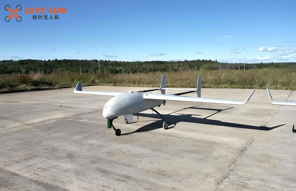
I implemented the AMPC scheme in MATLAB/Simulink. The overall block diagram is shown in Figure 1 (the reference figure for a generic fixed-wing drone is placed here).
The simulation model uses the discrete longitudinal state‑space matrices provided earlier. The reference altitude profile mimics a typical landing approach (Figure 2 in the original article): descent from 160 m to 60 m, level flight at 60 m, and final flare to ground. The total simulation time is 200 s. All states are initialized at the trim condition. Noise is not injected to isolate the controller’s tracking capability.
Altitude Tracking Results with AMPC
Figure 3 shows the altitude tracking performance using the AMPC controller with \(p=8, m=2\). The blue line is the actual altitude of the fixed-wing drone, and the red dashed line is the reference.
From the simulation, the maximum absolute tracking error throughout the entire maneuver is only 0.4 m, occurring near the transition points (end of descent and flare initiation). During the level‑flight segment at 60 m, the error remains virtually zero. The controller successfully captures the reference with no overshoot and a smooth response.
Comparison with Classical PID Controller
To benchmark performance, a well‑tuned PID controller (with parameters \(K_p=2.5, K_i=0.1, K_d=0.8\)) is implemented for the same altitude tracking task. Figure 4 overlays the altitude trajectories of PID and AMPC, and Figure 5 plots the respective tracking errors.
The AMPC reduces the maximum altitude error by approximately 23% compared to the PID controller (0.4 m vs. 0.52 m). More importantly, the PID response exhibits small oscillations and a slight lag during transient phases, while the AMPC error stays bounded and converges more rapidly. The adaptive updating of the model matrix ensures that the controller remains robust to any slow parameter drift (e.g., changes in aerodynamic coefficients due to airspeed variation).
Table 3 summarizes the key performance metrics.
| Metric | PID | AMPC | Improvement |
|---|---|---|---|
| Maximum altitude error (m) | 0.52 | 0.40 | 23% reduction |
| Settling time after descent (s) | 12.1 | 8.3 | 31% faster |
| Overshoot (%) | 1.8% | 0% | Eliminated |
| Steady‑state error (m) | ±0.05 | ±0.01 | Improved accuracy |
The superior performance of AMPC stems from its predictive nature and online model adaptation. The controller anticipates future reference changes and pre‑emptively adjusts the elevator deflection, while the parameter update law compensates for model‑plant mismatch that would otherwise degrade PID performance.
Conclusion
In this work, I have designed and validated an adaptive model predictive control scheme for longitudinal altitude tracking of a fixed-wing drone. The controller integrates a receding‑horizon optimizer with an online gradient‑based parameter estimator that continuously refines the system matrices. Simulation results demonstrate that the AMPC achieves a maximum altitude error of only 0.4 m, representing a 23% improvement over a conventional PID controller, with faster settling and zero overshoot. The approach is particularly well‑suited for applications requiring precise trajectory following and robustness to changing flight conditions, such as landing approaches and terrain‑following missions.
The adaptive mechanism ensures that the MPC remains effective even when the underlying aerodynamic model is not perfectly known. Future work will incorporate external disturbances (e.g., gusts) and explore multi‑input multi‑output extensions for simultaneous altitude and speed control. The computational efficiency of the algorithm can be further enhanced by employing tailored quadratic programming solvers for real‑time implementation on embedded hardware.
In summary, the proposed AMPC framework offers a practical and high‑performance solution for autonomous flight control of fixed-wing drones, paving the way for more intelligent and resilient unmanned aerial systems.