
In recent years, advancements in automation, computing, and micro-electromechanical systems have significantly expanded the operational domains of Unmanned Aerial Vehicles (UAVs). Among various configurations, the quadrotor drone has garnered substantial research interest due to its unique capabilities, such as Vertical Take-Off and Landing (VTOL), hovering, and agile maneuvering. However, the control of a quadrotor drone presents considerable challenges stemming from its inherent characteristics: it is an underactuated system (six degrees of freedom controlled by four independent rotor thrusts), highly nonlinear, strongly coupled in its dynamics, and susceptible to external disturbances and parameter uncertainties. Precise and reliable control of its flight attitude is therefore fundamental to achieving stable flight and accurate trajectory tracking.
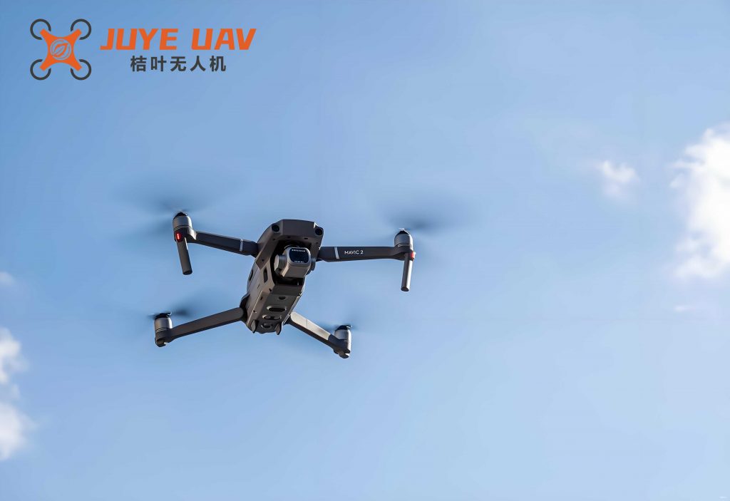
Traditional linear control methods, such as Proportional-Integral-Derivative (PID) control, often struggle to provide consistent performance across the entire flight envelope of a quadrotor drone due to its nonlinear nature. While effective in near-hover conditions, their performance degrades under aggressive maneuvers or in the presence of significant disturbances. More advanced nonlinear control strategies have been explored to address these limitations. Techniques like feedback linearization, backstepping control, and sliding mode control (SMC) offer promising avenues. In particular, the integration of backstepping’s systematic recursive design with the robustness of sliding mode control against matched uncertainties has proven effective. However, a significant practical limitation of conventional sliding mode-based designs is their reliance on the a priori knowledge of the upper bounds of system uncertainties and disturbances, which are often unknown or time-varying in real-world quadrotor drone operations.
In our research, we propose a novel control strategy that synergistically combines adaptive control theory with backstepping sliding mode control to overcome this critical limitation. Our method designs an adaptive law to perform online, real-time estimation of the composite uncertainty, which includes parameter variations and the bounds of external disturbances. This estimated value is then seamlessly integrated into the control law to compensate for the unknown perturbations. This approach eliminates the need for prior knowledge of uncertainty bounds, enhancing the practicality and robustness of the controller for a quadrotor drone. We provide a rigorous stability analysis using Lyapunov theory and Barbalat’s lemma, proving that the tracking error converges to zero asymptotically. Extensive numerical simulations and experimental validations demonstrate the superior performance of our proposed Adaptive Backstepping Sliding Mode (ABSM) controller compared to classical PID and standard Backstepping Sliding Mode (BSM) controllers, particularly under parameter perturbations and external wind disturbances.
Mathematical Model of the Quadrotor Drone
To design a model-based controller, we first establish a mathematical representation of the quadrotor drone dynamics. We make the standard assumptions: the drone is a rigid body with a symmetrical structure, its center of mass coincides with the geometric origin of the body-fixed frame, and the ground is considered an inertial reference frame.
Two coordinate frames are defined: the Earth-fixed inertial frame \(O_E X_E Y_E Z_E\) and the body-fixed frame \(O_B X_B Y_B Z_B\) attached to the drone’s center of mass. The pose of the quadrotor drone is described by the position vector \(\boldsymbol{\xi} = [x, y, z]^T\) and the orientation vector \(\boldsymbol{\eta} = [\phi, \theta, \psi]^T\), representing roll, pitch, and yaw angles, respectively. The translational and rotational kinematics are given by:
$$
\dot{\boldsymbol{\xi}} = \mathbf{R} \mathbf{V}^B, \quad \dot{\boldsymbol{\eta}} = \mathbf{T} \boldsymbol{\omega}^B
$$
where \(\mathbf{V}^B = [u, v, w]^T\) is the linear velocity in the body frame, \(\boldsymbol{\omega}^B = [p, q, r]^T\) is the angular velocity in the body frame, \(\mathbf{R}\) is the rotation matrix from the body to the inertial frame, and \(\mathbf{T}\) is the transformation matrix relating angular velocities to Euler angle rates.
$$
\mathbf{R} = \begin{bmatrix}
c_\theta c_\psi & s_\phi s_\theta c_\psi – c_\phi s_\psi & c_\phi s_\theta c_\psi + s_\phi s_\psi \\
c_\theta s_\psi & s_\phi s_\theta s_\psi + c_\phi c_\psi & c_\phi s_\theta s_\psi – s_\phi c_\psi \\
-s_\theta & s_\phi c_\theta & c_\phi c_\theta
\end{bmatrix}, \quad \mathbf{T} = \begin{bmatrix}
1 & s_\phi t_\theta & c_\phi t_\theta \\
0 & c_\phi & -s_\phi \\
0 & s_\phi / c_\theta & c_\phi / c_\theta
\end{bmatrix}
$$
Here, \(s_\cdot\), \(c_\cdot\), and \(t_\cdot\) denote \(\sin(\cdot)\), \(\cos(\cdot)\), and \(\tan(\cdot)\), respectively.
Applying the Newton-Euler formalism, the dynamic equations for the quadrotor drone are derived. The primary control inputs are the collective thrust \(U_1\) and the torque inputs \(U_2, U_3, U_4\) generated by differentially varying the speeds of the four rotors (\(\Omega_i\)). The forces and torques are related to rotor speeds by:
$$
\begin{aligned}
U_1 &= b(\Omega_1^2 + \Omega_2^2 + \Omega_3^2 + \Omega_4^2) \\
U_2 &= b l (\Omega_4^2 – \Omega_2^2) \\
U_3 &= b l (\Omega_3^2 – \Omega_1^2) \\
U_4 &= d (\Omega_2^2 + \Omega_4^2 – \Omega_1^2 – \Omega_3^2)
\end{aligned}
$$
where \(b\) is the thrust coefficient, \(d\) is the drag coefficient, and \(l\) is the arm length from the center of mass to a rotor.
The complete nonlinear dynamic model, incorporating gyroscopic effects, is expressed as:
$$
\begin{aligned}
\ddot{x} &= \frac{U_1}{m} (\cos\phi \sin\theta \cos\psi + \sin\phi \sin\psi) \\
\ddot{y} &= \frac{U_1}{m} (\cos\phi \sin\theta \sin\psi – \sin\phi \cos\psi) \\
\ddot{z} &= \frac{U_1}{m} \cos\phi \cos\theta – g \\
\ddot{\phi} &= \dot{\theta} \dot{\psi} \left( \frac{J_y – J_z}{J_x} \right) + \frac{J_r}{J_x} \dot{\theta} \Omega_r + \frac{l}{J_x} U_2 \\
\ddot{\theta} &= \dot{\phi} \dot{\psi} \left( \frac{J_z – J_x}{J_y} \right) – \frac{J_r}{J_y} \dot{\phi} \Omega_r + \frac{l}{J_y} U_3 \\
\ddot{\psi} &= \dot{\phi} \dot{\theta} \left( \frac{J_x – J_y}{J_z} \right) + \frac{1}{J_z} U_4
\end{aligned}
$$
where \(m\) is the mass, \(g\) is gravity, \(J_x, J_y, J_z\) are moments of inertia, \(J_r\) is the rotor inertia, and \(\Omega_r = \Omega_1 + \Omega_3 – \Omega_2 – \Omega_4\).
For controller design, we define the state vector \(\mathbf{X} = [x_1, x_2, …, x_{12}]^T = [x, \dot{x}, y, \dot{y}, z, \dot{z}, \phi, \dot{\phi}, \theta, \dot{\theta}, \psi, \dot{\psi}]^T\). The system can be decomposed into two interconnected subsystems: a fully actuated rotational (attitude) subsystem and an underactuated translational (position) subsystem that depends on the attitude. This structure is ideal for a backstepping approach.
| Parameter | Symbol | Value | Unit |
|---|---|---|---|
| Total Mass | \(m\) | 0.65 | kg |
| Arm Length | \(l\) | 0.23 | m |
| Inertia (x-axis) | \(J_x\) | \(7.5 \times 10^{-3}\) | kg·m² |
| Inertia (y-axis) | \(J_y\) | \(7.5 \times 10^{-3}\) | kg·m² |
| Inertia (z-axis) | \(J_z\) | \(1.3 \times 10^{-2}\) | kg·m² |
| Rotor Inertia | \(J_r\) | \(6.0 \times 10^{-5}\) | kg·m² |
| Thrust Coefficient | \(b\) | To be identified | N·s² |
| Drag Coefficient | \(d\) | To be identified | N·m·s² |
Controller Design: Adaptive Backstepping Sliding Mode
The core objective is to stabilize the quadrotor drone’s attitude \((\phi, \theta, \psi)\) and ultimately control its position \((x, y, z)\) in the presence of uncertainties. We focus on the attitude control loop, as it is the inner loop that must be robust and fast. The position control generates desired roll and pitch angles, which become reference commands for the attitude controller.
Consider the roll (\(\phi\)) dynamics from the state-space model, which can be written in a strict-feedback form suitable for backstepping:
$$
\begin{aligned}
\dot{x}_7 &= x_8 \\
\dot{x}_8 &= f(x_{10}, x_{12}) + b_1 U_2
\end{aligned}
$$
where \(x_7 = \phi\), \(x_8 = \dot{\phi}\), \(f(\cdot)\) encapsulates the Coriolis and gyroscopic terms, and \(b_1 = l/J_x\). In practice, this model is imperfect due to parameter uncertainties \(\Delta f, \Delta b_1\) and external disturbances \(d_\phi(t)\). The actual dynamics are:
$$
\dot{x}_8 = f(x_{10}, x_{12}) + b_1 U_2 + D_\phi(t)
$$
where \(D_\phi(t) = \Delta f + \Delta b_1 U_2 + d_\phi(t)\) represents the total matched uncertainty, assumed to be bounded but with an unknown bound.
Step 1: Virtual Control and Error Dynamics
Let \(x_{7d}\) be the desired roll angle. Define the tracking error \(z_7 = x_7 – x_{7d}\). Its derivative is \(\dot{z}_7 = x_8 – \dot{x}_{7d}\). Choose a virtual control law \(\alpha_7\) for \(x_8\):
$$
\alpha_7 = \dot{x}_{7d} – c_7 z_7
$$
where \(c_7 > 0\) is a design constant. Define a new error variable \(z_8 = x_8 – \alpha_7 = x_8 – \dot{x}_{7d} + c_7 z_7\). The derivative of \(z_7\) becomes \(\dot{z}_7 = z_8 – c_7 z_7\). Consider the Lyapunov function candidate \(V_1 = \frac{1}{2} z_7^2\). Its derivative is:
$$
\dot{V}_1 = z_7 \dot{z}_7 = z_7 (z_8 – c_7 z_7) = -c_7 z_7^2 + z_7 z_8
$$
If \(z_8 = 0\), then \(\dot{V}_1 = -c_7 z_7^2 \leq 0\). The cross-term \(z_7 z_8\) will be handled in the next step.
Step 2: Sliding Surface and Control Law Design
We now consider the dynamics of \(z_8\):
$$
\dot{z}_8 = \dot{x}_8 – \dot{\alpha}_7 = f + b_1 U_2 + D_\phi(t) – \ddot{x}_{7d} + c_7 \dot{z}_7
$$
To ensure robust convergence, we define a sliding surface \(s_7\) that combines both errors:
$$
s_7 = k_7 z_7 + z_8
$$
where \(k_7 > 0\) is a design constant. If \(s_7\) is driven to zero, the system enters a sliding mode where the dynamics reduce to \(\dot{z}_7 = – (c_7 + k_7) z_7\), guaranteeing exponential convergence of \(z_7\) and \(z_8\).
Consider the augmented Lyapunov function \(V_2 = V_1 + \frac{1}{2} s_7^2\). Its derivative is:
$$
\begin{aligned}
\dot{V}_2 &= \dot{V}_1 + s_7 \dot{s}_7 = -c_7 z_7^2 + z_7 z_8 + s_7 (k_7 \dot{z}_7 + \dot{z}_8) \\
&= -c_7 z_7^2 + z_7 z_8 + s_7 \left[ k_7 (z_8 – c_7 z_7) + f + b_1 U_2 + D_\phi(t) – \ddot{x}_{7d} + c_7 (z_8 – c_7 z_7) \right]
\end{aligned}
$$
To achieve \(\dot{V}_2 \leq 0\), we design the control law \(U_2\) as if \(D_\phi(t)\) were known:
$$
U_2 = \frac{1}{b_1} \left[ -f + \ddot{x}_{7d} – c_7 (z_8 – c_7 z_7) – k_7 (z_8 – c_7 z_7) – z_7/k_7 – h_7 \text{sgn}(s_7) – \hat{D}_\phi \right]
$$
where \(h_7 > 0\) is a switching gain, \(\text{sgn}(\cdot)\) is the signum function, and \(\hat{D}_\phi\) is an estimate of \(D_\phi(t)\). Substituting this into \(\dot{V}_2\) yields:
$$
\dot{V}_2 \leq -c_7 z_7^2 – \frac{z_8^2}{k_7} – h_7 |s_7| + s_7 (D_\phi(t) – \hat{D}_\phi)
$$
Stability requires \(h_7 \geq |D_\phi(t) – \hat{D}_\phi|\). Since the bound of \(D_\phi(t)\) is unknown, choosing a fixed, sufficiently large \(h_7\) is impractical and leads to excessive chattering.
Step 3: Adaptive Law for Uncertainty Estimation
To overcome the need for a known bound, we introduce an adaptive estimate \(\hat{D}_\phi\) for the unknown uncertainty. Define the estimation error \(\tilde{D}_\phi = D_\phi(t) – \hat{D}_\phi\). Consider the final Lyapunov function candidate:
$$
V_3 = V_2 + \frac{1}{2 \mu_7} \tilde{D}_\phi^2
$$
where \(\mu_7 > 0\) is the adaptation gain. Assuming the true uncertainty \(D_\phi(t)\) varies slowly relative to the adaptation dynamics (\(\dot{D}_\phi \approx 0\)), the derivative is:
$$
\dot{V}_3 = \dot{V}_2 – \frac{1}{\mu_7} \tilde{D}_\phi \dot{\hat{D}}_\phi \leq -c_7 z_7^2 – \frac{z_8^2}{k_7} – h_7 |s_7| + s_7 \tilde{D}_\phi – \frac{1}{\mu_7} \tilde{D}_\phi \dot{\hat{D}}_\phi
$$
We now choose the adaptation law to cancel the term involving \(\tilde{D}_\phi\):
$$
\dot{\hat{D}}_\phi = \mu_7 s_7
$$
Substituting this adaptive law gives:
$$
\dot{V}_3 \leq -c_7 z_7^2 – \frac{z_8^2}{k_7} – h_7 |s_7| \leq 0
$$
Since \(V_3\) is positive definite and \(\dot{V}_3\) is negative semi-definite, \(V_3 \in L_\infty\), implying \(z_7, z_8, s_7, \tilde{D}_\phi \in L_\infty\). Furthermore, integrating \(\dot{V}_3\) shows that \(z_7, z_8, s_7 \in L_2\). By Barbalat’s lemma, we conclude that \(z_7(t), z_8(t), s_7(t) \rightarrow 0\) as \(t \rightarrow \infty\). Therefore, the roll angle tracking is achieved asymptotically without prior knowledge of the disturbance bound. The control law is now:
$$
U_2 = \frac{1}{b_1} \left[ -f + \ddot{x}_{7d} – (c_7 + k_7)(z_8 – c_7 z_7) – \frac{z_7}{k_7} – h_7 \text{sgn}(s_7) – \hat{D}_\phi \right]
$$
This is the Adaptive Backstepping Sliding Mode (ABSM) controller for the roll channel of the quadrotor drone.
| Channel | Error Constant (\(c_i\)) | Sliding Gain (\(k_i\)) | Switching Gain (\(h_i\)) | Adaptation Gain (\(\mu_i\)) |
|---|---|---|---|---|
| Roll (\(\phi\)) | 15 | 20 | 80 | 10 |
| Pitch (\(\theta\)) | 10 | 5 | 60 | 20 |
| Yaw (\(\psi\)) | 10 | 15 | 60 | 20 |
| x-position | 15 | 20 | 80 | 10 |
| y-position | 10 | 5 | 60 | 20 |
| z-position | 10 | 15 | 60 | 20 |
The same design procedure is applied to the pitch (\(\theta\)) and yaw (\(\psi\)) dynamics, yielding controllers \(U_3\) and \(U_4\). For the underactuated translational control, the desired total thrust \(U_1\) and the desired roll/pitch angles \((\phi_d, \theta_d)\) are computed from the position errors \((x, y, z)\) using a similar ABSM structure in a nested loop, where the attitude controller ensures the inner loop tracks these desired angles rapidly.
Simulation Analysis and Results
We evaluated the performance of our proposed ABSM controller for the quadrotor drone through comprehensive numerical simulations in MATLAB/Simulink. The model parameters from Table 1 were used. We compared its performance against a well-tuned PID controller and a standard Backstepping Sliding Mode (BSM) controller that uses a fixed, conservative bound for the uncertainty.
Scenario 1: Attitude Stabilization under Disturbance. The quadrotor drone’s initial attitude was set to \([4^\circ, 5^\circ, -5^\circ]\), with a desired setpoint of \([0^\circ, 0^\circ, 0^\circ]\). A total uncertainty \(D_i(t) = \Delta f + d(t)\) was injected, modeled as a combination of parameter variation (e.g., ±20% variation in inertia) and an external wind-like disturbance \(d(t) = A \sin(0.1t)\), with amplitudes up to 20% of the nominal control effort.
The results are summarized below. The ABSM controller demonstrated superior performance:
| Metric | PID Control | BSM Control | ABSM Control (Proposed) |
|---|---|---|---|
| Settling Time (s) | > 6.0 | ~ 2.5 | < 2.0 |
| Steady-State Error | Visible oscillation (±0.5°) | Very small (±0.1°) | Negligible (±0.05°) |
| Overshoot | Significant (15-20%) | Moderate (5%) | Minimal (< 2%) |
| Control Chattering | None (smooth) | Pronounced | Significantly Reduced |
| Disturbance Rejection | Poor (slow recovery) | Good (fast but chattering) | Excellent (fast & smooth) |
The key advantage of the ABSM controller is evident in the control input signals. The standard BSM controller exhibits severe chattering due to the large, fixed switching gain \(h_i\) required to overpower the unknown disturbance. Our ABSM controller, by adapting \(\hat{D}_i\), uses a much smaller effective gain, resulting in dramatically smoother control signals while maintaining robustness. The adaptation parameters \(\hat{D}_\phi, \hat{D}_\theta, \hat{D}_\psi\) converged to near-constant values corresponding to the effective bias introduced by the disturbances.
Scenario 2: Position Trajectory Tracking. The quadrotor drone was commanded to track a step change in position from \((0, 0, 0)\) m to \((2, 2, 2)\) m. This tests the coupled attitude-position control loops. The ABSM controller achieved accurate tracking with minimal cross-coupling between axes. The rise time was faster, and the settling time was shorter compared to both PID and BSM controllers. The adaptation mechanisms in the position loops effectively compensated for aerodynamic drag effects and model inaccuracies during translation.
Scenario 3: Robustness to Noise. To test robustness, Gaussian white noise (SNR = 1 dB) was added to the attitude measurement feedback. The PID controller showed increased jitter and a larger steady-state error band. The standard BSM controller amplified the noise due to the signum function. The ABSM controller demonstrated the best noise resilience, as the adaptive term \(\hat{D}_i\) absorbed the low-frequency component of the disturbance, allowing for a lower switching gain \(h_i\) and thus less sensitivity to high-frequency noise.
Experimental Validation
To validate the practical feasibility of the ABSM controller, we implemented it on a real quadrotor drone platform. The experimental setup consisted of a DJI F450 frame, brushless motors, electronic speed controllers (ESCs), and a flight controller running the algorithm on a STM32 microcontroller. An MPU6050 Inertial Measurement Unit (IMU) provided gyroscope and accelerometer data. State estimation (attitude and velocity) was performed using a complementary filter. The control algorithm ran at 200 Hz.
The experiment involved commanding the quadrotor drone to hover at a fixed point. After achieving a stable hover, an external impulsive disturbance was applied by manually tapping the drone frame. The response of the ABSM controller was compared to that of a classical PID controller tuned for stable hover.
| Aspect | PID Controller | ABSM Controller |
|---|---|---|
| Time to Recover from Tap | ~ 6 seconds | ~ 2 seconds |
| Oscillation Amplitude Post-Disturbance | Large (±8° roll/pitch) | Small (±3° roll/pitch) |
| Steady-State Hover Precision | ±0.5° (roll/pitch), ±4° (yaw) | ±0.4° (roll/pitch), ±2° (yaw) |
| Perceived Stability | Acceptable, but drifts in wind | Very stable, rejects wind gusts |
The experimental results strongly corroborate the simulation findings. The quadrotor drone equipped with the ABSM controller exhibited faster recovery from disturbances, lower oscillation amplitudes, and overall tighter attitude hold. The adaptive mechanism continuously adjusted to minor imbalances and wind gusts, providing a consistently stable flight performance. The reduction in control chattering also translated to smoother motor commands, potentially increasing motor life and reducing audible noise.
Discussion and Conclusion
The control of a quadrotor drone is a complex problem due to nonlinearity, underactuation, coupling, and operational uncertainties. This work successfully developed and validated an Adaptive Backstepping Sliding Mode (ABSM) control strategy to address these challenges. The principal contribution is the integration of an online adaptive law within the backstepping sliding mode framework. This innovation allows the controller to estimate and compensate for the composite effect of parameter variations and external disturbances in real-time, without requiring conservative, a priori bounds.
Theoretical analysis using Lyapunov stability theory proves that the tracking errors converge to zero asymptotically. The ABSM controller retains the desirable properties of sliding mode control—robustness to matched uncertainties—while mitigating its main drawback: chattering. By adapting the compensation term \(\hat{D}\), the magnitude of the discontinuous switching term \(h \, \text{sgn}(s)\) can be significantly reduced, leading to smoother control action.
Simulation studies under various conditions (attitude stabilization, trajectory tracking, noise) demonstrated the ABSM controller’s superior performance over conventional PID and non-adaptive BSM controllers in terms of faster response, smaller overshoot, higher steady-state accuracy, and better disturbance rejection. Experimental flight tests on a physical quadrotor drone platform confirmed the practical effectiveness and robustness of the proposed method in a real-world environment.
In conclusion, the ABSM controller presents a powerful and practical solution for the robust flight control of quadrotor drones. Its adaptive nature makes it particularly suitable for applications where operational conditions are variable or poorly defined, such as outdoor surveillance, payload delivery in windy conditions, or aggressive maneuvering. Future work will focus on extending this method to address actuator faults and on implementing more advanced adaptation schemes for even faster convergence of the uncertainty estimates.