
The operational reliability of quadrotor drones is paramount for their widespread adoption in both civilian and military applications, ranging from aerial photography and payload delivery to surveillance and inspection. As these systems are often deployed in dynamic and potentially harsh environments, they are susceptible to various faults, with actuator faults being among the most critical due to their direct impact on flight control and stability. Early and accurate detection of such faults is therefore essential to initiate safety protocols, implement fault-tolerant control, or execute emergency landings, thereby preventing catastrophic failures. This article presents a robust model-based fault detection (FD) scheme for quadrotor drones, specifically targeting actuator faults. The proposed methodology leverages an Unknown Input Observer (UIO) for disturbance decoupling and utilizes zonotopes, a specific class of convex sets, to generate adaptive detection thresholds, enabling reliable fault diagnosis even in the presence of bounded modeling uncertainties and measurement noise.
The core challenge in model-based FD for quadrotor drones lies in distinguishing the effects of a fault from those of inherent system uncertainties, external disturbances, and sensor noise. A fault detection residual, which is the difference between the measured system output and the output estimated by a mathematical model, is typically generated. Under normal (fault-free) conditions, this residual should remain close to zero or within a predictable bound. A fault is declared when the residual deviates significantly from this nominal behavior. However, the residual is also affected by unknown inputs and noise, which can lead to false alarms or missed detections if not properly accounted for. The approach detailed herein addresses this by designing an observer that is completely decoupled from a specific class of disturbances (unknown inputs) and by employing set-membership methods to compute guaranteed bounds for the residual under all possible uncertainties.
1. Dynamic Modeling of the Quadrotor Drone
To design a model-based fault detection scheme, an accurate yet tractable mathematical model of the quadrotor drone is required. The standard six-degree-of-freedom (6-DOF) nonlinear model is derived using Newton-Euler formalism. For the purpose of fault detection focused on the attitude control loop, and considering hover or near-hover flight conditions typical for many missions, the complex nonlinear model can be effectively linearized. The following standard assumptions are made to simplify the model derivation:
| Assumption | Description |
|---|---|
| 1. Rigid Body Structure | The quadrotor drone is assumed to be a rigid body with constant mass and symmetrical structure about its center of mass. |
| 2. Planar Symmetry | The inertia matrix is diagonal, and the center of gravity coincides with the geometric center of the body. |
| 3. Small Attitude Angles | For linearization, the roll ($\phi$), pitch ($\theta$), and yaw ($\psi$) angles are considered small ($< 5^\circ$). |
| 4. Linear Thrust/Torque | The thrust and torque generated by each rotor are proportional to the square of its rotational speed, which can be linearized around an operating point. |
Under these assumptions, the linearized equations describing the attitude dynamics (roll, pitch, yaw) of the quadrotor drone can be derived. Let $\boldsymbol{x} = [\theta, \phi, \psi, \dot{\theta}, \dot{\phi}, \dot{\psi}]^T$ represent the state vector comprising the three Euler angles and their angular rates. The control input vector $\boldsymbol{u} = [\delta u_1, \delta u_2, \delta u_3, \delta u_4]^T$ represents the deviation of the motor speed commands from their hover equilibrium values. The linearized, continuous-time state-space model is given by:
$$
\dot{\boldsymbol{x}}(t) = \boldsymbol{A}_c \boldsymbol{x}(t) + \boldsymbol{B}_c \boldsymbol{u}(t)
$$
$$
\boldsymbol{y}(t) = \boldsymbol{C} \boldsymbol{x}(t)
$$
where $\boldsymbol{y} = [\theta, \phi, \psi]^T$ is the measured output, typically obtained from an Inertial Measurement Unit (IMU). The matrices $\boldsymbol{A}_c$ and $\boldsymbol{B}_c$ are system matrices whose elements are functions of the quadrotor drone’s physical parameters such as moments of inertia ($J_{xx}, J_{yy}, J_{zz}$), thrust coefficient ($k_f$), drag coefficient ($k_m$), and the distance from the center of mass to each rotor ($l$).
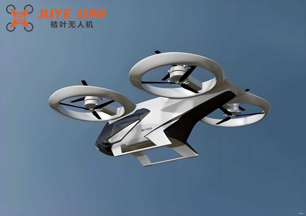
For digital implementation of the observer and fault detection algorithm, the continuous-time model must be discretized. Using a zero-order hold on the inputs and a sampling period $T_s$, the discrete-time state-space model of the healthy quadrotor drone system is obtained:
$$
\boldsymbol{x}_{k+1} = \boldsymbol{G} \boldsymbol{x}_k + \boldsymbol{K} \boldsymbol{u}_k + \boldsymbol{D}_1 \boldsymbol{\omega}_k
$$
$$
\boldsymbol{y}_k = \boldsymbol{C} \boldsymbol{x}_k + \boldsymbol{D}_2 \boldsymbol{\upsilon}_k
$$
Here, $\boldsymbol{G} = e^{\boldsymbol{A}_c T_s}$ and $\boldsymbol{K} = \int_{0}^{T_s} e^{\boldsymbol{A}_c \tau} d\tau \boldsymbol{B}_c$ are the discrete-time system and input matrices, respectively. The terms $\boldsymbol{D}_1 \boldsymbol{\omega}_k$ and $\boldsymbol{D}_2 \boldsymbol{\upsilon}_k$ are explicitly included to account for process disturbances (e.g., wind gusts, model inaccuracies) and measurement noise, respectively. These signals are assumed to be unknown but bounded, belonging to known sets: $\boldsymbol{\omega}_k \in \mathcal{W}$ and $\boldsymbol{\upsilon}_k \in \mathcal{V}$. This boundedness assumption is crucial for the subsequent set-membership approach using zonotopes.
2. Actuator Fault Modeling for the Quadrotor Drone
An actuator fault in a quadrotor drone typically corresponds to an abnormal behavior of one or more of its four rotors. This could result from physical damage, electronic speed controller (ESC) failure, motor wear, or battery issues. The effect of an actuator fault can be modeled as an additive term in the discrete-time state equation. Considering a fault affecting a single actuator at a time (a common hypothesis in initial fault isolation), the faulty system model becomes:
$$
\boldsymbol{x}_{k+1} = \boldsymbol{G} \boldsymbol{x}_k + \boldsymbol{K} \boldsymbol{u}_k + \boldsymbol{F}_i f_{i,k} + \boldsymbol{D}_1 \boldsymbol{\omega}_k
$$
$$
\boldsymbol{y}_k = \boldsymbol{C} \boldsymbol{x}_k + \boldsymbol{D}_2 \boldsymbol{\upsilon}_k
$$
In this model, $f_{i,k}$ represents the fault signal associated with the $i$-th actuator ($i \in \{1,2,3,4\}$). The vector $\boldsymbol{F}_i$ is the $i$-th column of the fault distribution matrix $\boldsymbol{F}$, which defines how a fault in actuator $i$ influences the system states. For a quadrotor drone, $\boldsymbol{F}$ is closely related to the input matrix $\boldsymbol{K}$, as a fault directly affects the forces and torques applied to the airframe. The fault signal $f_{i,k}$ can represent different types of failures commonly encountered in quadrotor drone operations:
| Fault Type | Mathematical Model | Physical Interpretation |
|---|---|---|
| Abrupt (Bias) Fault | $f_{i,k} = \begin{cases} 0 & k < k_{fault} \\ \beta & k \ge k_{fault} \end{cases}$ | Sudden loss of partial thrust/torque (e.g., motor damage, ESC lock). |
| Incipient (Drift) Fault | $f_{i,k} = \begin{cases} 0 & k < k_{fault} \\ \alpha \cdot (k – k_{fault}) & k \ge k_{fault} \end{cases}$ | Gradual degradation of performance (e.g., motor wear, propeller erosion). |
| Loss of Effectiveness | $f_{i,k}$ modifies $\boldsymbol{K}$ column: $(\boldsymbol{K}_i \cdot (1 – f_{i,k}))$ | The actuator provides only a fraction of its commanded input. |
The primary objective of the fault detection system for the quadrotor drone is to generate an alarm when the magnitude or behavior of any $f_{i,k}$ deviates from zero, indicating an actuator anomaly.
3. Fault Detection Methodology
The proposed fault detection framework for the quadrotor drone consists of two main components: 1) a bank of Unknown Input Observers (UIOs) designed to be insensitive to disturbances $\boldsymbol{\omega}_k$, and 2) a zonotope-based residual evaluation mechanism that determines adaptive detection thresholds.
3.1. Unknown Input Observer Design
The goal of the UIO is to estimate the states of the quadrotor drone while completely decoupling the estimation error from the unknown input disturbance $\boldsymbol{\omega}_k$. This ensures that the residual is primarily sensitive to faults and measurement noise, but not to disturbances, significantly reducing false alarms. The standard UIO structure for the discrete-time system is given by:
$$
\boldsymbol{z}_{k+1} = \boldsymbol{P} \boldsymbol{z}_k + \boldsymbol{J} \boldsymbol{u}_k + \boldsymbol{L} \boldsymbol{y}_k
$$
$$
\hat{\boldsymbol{x}}_k = \boldsymbol{z}_k + \boldsymbol{Q} \boldsymbol{y}_k
$$
where $\hat{\boldsymbol{x}}_k$ is the state estimate, and $\boldsymbol{z}_k$ is the internal observer state. The matrices $\boldsymbol{P}, \boldsymbol{J}, \boldsymbol{L},$ and $\boldsymbol{Q}$ are designed to satisfy the following conditions for perfect unknown input decoupling and stable error dynamics:
1. Disturbance Decoupling Condition: $(\boldsymbol{I} – \boldsymbol{Q}\boldsymbol{C})\boldsymbol{D}_1 = \boldsymbol{0}$. This ensures the disturbance term is eliminated from the state estimation error dynamics. A solution for $\boldsymbol{Q}$ exists if and only if $\text{rank}(\boldsymbol{C}\boldsymbol{D}_1) = \text{rank}(\boldsymbol{D}_1)$.
2. State Estimation Error Dynamics: The estimation error $\boldsymbol{e}_k = \boldsymbol{x}_k – \hat{\boldsymbol{x}}_k$ evolves according to:
$$
\boldsymbol{e}_{k+1} = (\boldsymbol{G} – \boldsymbol{Q}\boldsymbol{C}\boldsymbol{G} – \boldsymbol{L}_1\boldsymbol{C})\boldsymbol{e}_k + [(\boldsymbol{I}-\boldsymbol{Q}\boldsymbol{C})\boldsymbol{D}_1]\boldsymbol{\omega}_k – \boldsymbol{L}_1\boldsymbol{D}_2\boldsymbol{\upsilon}_k – \boldsymbol{Q}\boldsymbol{D}_2\boldsymbol{\upsilon}_{k+1}
$$
By satisfying condition 1, the term with $\boldsymbol{\omega}_k$ vanishes. Defining $\boldsymbol{P} = \boldsymbol{G} – \boldsymbol{Q}\boldsymbol{C}\boldsymbol{G} – \boldsymbol{L}_1\boldsymbol{C}$ and $\boldsymbol{L} = \boldsymbol{L}_1 + \boldsymbol{P}\boldsymbol{Q}$, the error dynamics simplify to:
$$
\boldsymbol{e}_{k+1} = \boldsymbol{P} \boldsymbol{e}_k – \boldsymbol{L}_1\boldsymbol{D}_2\boldsymbol{\upsilon}_k – \boldsymbol{Q}\boldsymbol{D}_2\boldsymbol{\upsilon}_{k+1}
$$
3. Stability: The matrix $\boldsymbol{P}$ must be Schur stable (all eigenvalues inside the unit circle). The gain matrix $\boldsymbol{L}_1$ can be designed via pole placement or LMI techniques to achieve desired convergence rates for the quadrotor drone’s state estimates.
The output residual $\boldsymbol{r}_k$ is then defined as a weighted function of the output estimation error:
$$
\boldsymbol{r}_k = \boldsymbol{V} (\boldsymbol{y}_k – \boldsymbol{C}\hat{\boldsymbol{x}}_k) = \boldsymbol{V} (\boldsymbol{C}\boldsymbol{e}_k + \boldsymbol{D}_2\boldsymbol{\upsilon}_k)
$$
where $\boldsymbol{V}$ is a suitable residual weighting matrix.
3.2. Zonotope-based Adaptive Thresholding
Even after disturbance decoupling, the residual $\boldsymbol{r}_k$ is affected by measurement noise $\boldsymbol{\upsilon}_k$ and the propagated effect of past noise through the error dynamics. To reliably detect faults in the quadrotor drone, we need to determine the set of all possible residual values under fault-free conditions, considering all admissible noise sequences. This is where zonotopes are employed.
A zonotope $\mathcal{Z}$ is a convex, centrally symmetric polytope defined as the linear image of a hypercube:
$$
\mathcal{Z} = \langle \boldsymbol{c}, \boldsymbol{H} \rangle = \{ \boldsymbol{c} + \boldsymbol{H} \boldsymbol{\xi} : \boldsymbol{\xi} \in [-1, 1]^p \}
$$
where $\boldsymbol{c} \in \mathbb{R}^n$ is the center, and $\boldsymbol{H} \in \mathbb{R}^{n \times p}$ is the generator matrix. The key operations for propagating uncertainty sets through linear dynamics are straightforward for zonotopes:
$$
\boldsymbol{L} \cdot \langle \boldsymbol{c}, \boldsymbol{H} \rangle = \langle \boldsymbol{L}\boldsymbol{c}, \boldsymbol{L}\boldsymbol{H} \rangle, \quad \langle \boldsymbol{c}_1, \boldsymbol{H}_1 \rangle \oplus \langle \boldsymbol{c}_2, \boldsymbol{H}_2 \rangle = \langle \boldsymbol{c}_1+\boldsymbol{c}_2, [\boldsymbol{H}_1 \ \boldsymbol{H}_2] \rangle
$$
Given the noise boundedness assumptions $\boldsymbol{\upsilon}_k \in \mathcal{V} = \langle \boldsymbol{0}, \boldsymbol{H}_{\upsilon} \rangle$ and an initial estimation error bounded in $\boldsymbol{e}_0 \in \mathcal{E}_0 = \langle \boldsymbol{0}, \boldsymbol{H}_{e,0} \rangle$, we can compute the guaranteed bound (zonotope) for the state estimation error and the residual at every time step $k$.
The recursion for the fault-free state estimation error zonotope $\mathcal{E}_k = \langle \boldsymbol{0}, \boldsymbol{H}_{e,k} \rangle$ is derived from the error dynamics:
$$
\boldsymbol{e}_{k+1} \in \boldsymbol{P} \mathcal{E}_k \oplus (-\boldsymbol{L}_1\boldsymbol{D}_2\mathcal{V}) \oplus (-\boldsymbol{Q}\boldsymbol{D}_2\mathcal{V})
$$
Therefore, the generator matrix update is:
$$
\boldsymbol{H}_{e,k+1} = [\boldsymbol{P}\boldsymbol{H}_{e,k} \ \ -\boldsymbol{L}_1\boldsymbol{D}_2\boldsymbol{H}_{\upsilon} \ \ -\boldsymbol{Q}\boldsymbol{D}_2\boldsymbol{H}_{\upsilon}]
$$
Subsequently, the fault-free residual zonotope $\mathcal{R}_k = \langle \boldsymbol{0}, \boldsymbol{H}_{r,k} \rangle$ is:
$$
\boldsymbol{r}_k \in \boldsymbol{V}\boldsymbol{C} \mathcal{E}_k \oplus \boldsymbol{V}\boldsymbol{D}_2\mathcal{V}
$$
with generator matrix:
$$
\boldsymbol{H}_{r,k} = [\boldsymbol{V}\boldsymbol{C}\boldsymbol{H}_{e,k} \ \ \boldsymbol{V}\boldsymbol{D}_2\boldsymbol{H}_{\upsilon}]
$$
To obtain a scalar threshold for each residual component $r^{(i)}_k$, we compute the interval hull (axis-aligned bounding box) of the zonotope $\mathcal{R}_k$. The interval for the $i$-th component is given by:
$$
\underline{r}^{(i)}_k = -\sum_{j=1}^{p} |\boldsymbol{H}_{r,k}[i,j]|, \quad \overline{r}^{(i)}_k = \sum_{j=1}^{p} |\boldsymbol{H}_{r,k}[i,j]|
$$
where $\boldsymbol{H}_{r,k}[i,j]$ is the $(i,j)$-th element of the generator matrix. The adaptive threshold interval for component $i$ at time $k$ is $[\underline{r}^{(i)}_k, \overline{r}^{(i)}_k]$.
The fault detection logic for the quadrotor drone is then straightforward: at each time step $k$, compute the actual residual $\boldsymbol{r}_k$ from the UIO and the measured outputs. For each component $i$, check:
$$
\text{If } r^{(i)}_k \notin [\underline{r}^{(i)}_k, \overline{r}^{(i)}_k] \Rightarrow \text{Fault Alarm for residual channel } i.
$$
This method provides a guaranteed no false-alarm property under the considered bounded-noise assumptions, meaning if no fault is present, the residual will never exceed the computed threshold. A violation is a conclusive indicator of a fault (or a violation of the noise bounds) in the quadrotor drone system.
4. Simulation Study on a Quadrotor Drone Model
To validate the effectiveness of the proposed fault detection scheme, a numerical simulation was conducted using a high-fidelity model of a quadrotor drone. The discrete-time system matrices ($\boldsymbol{G}, \boldsymbol{K}, \boldsymbol{C}$) were derived from the linearized dynamics around a hover condition with a sampling time $T_s = 0.01$ s. The disturbance and noise distribution matrices $\boldsymbol{D}_1, \boldsymbol{D}_2$ were defined to represent realistic uncertainty channels. The bounded noise sequences $\boldsymbol{\omega}_k$ and $\boldsymbol{\upsilon}_k$ were randomly generated within their respective zonotopic sets $\mathcal{W}$ and $\mathcal{V}$.
| Parameter | Symbol | Value |
|---|---|---|
| Sampling Time | $T_s$ | 0.01 s |
| Moment of Inertia (Roll) | $J_{xx}$ | 0.025 kg·m² |
| Moment of Inertia (Pitch) | $J_{yy}$ | 0.025 kg·m² |
| Moment of Inertia (Yaw) | $J_{zz}$ | 0.04 kg·m² |
| Thrust Coefficient | $k_f$ | 1.5e-5 N/(rad/s)² |
| Drag Coefficient | $k_m$ | 3e-7 Nm/(rad/s)² |
| Arm Length | $l$ | 0.2 m |
The UIO was designed according to the procedure in Section 3.1. The decoupling matrix $\boldsymbol{Q}$ was calculated, and the observer gain $\boldsymbol{L}_1$ was designed via pole placement to locate the poles of $\boldsymbol{P}$ at $[0.5, 0.55, 0.6, 0.65, 0.7, 0.75]$, ensuring fast and stable convergence for the quadrotor drone state estimates. The initial condition zonotope $\mathcal{E}_0$ was set based on typical initial estimation errors.
Fault Scenario: Two distinct actuator fault scenarios were simulated to test the robustness and sensitivity of the detector:
- Abrupt Fault in Actuator 1: At time $k=500$ (5 seconds), a sudden bias fault occurs: $f_{1,k} = 0.8$ for $k \ge 500$.
- Incipient Fault in Actuator 2: At time $k=500$, a slowly growing fault begins: $f_{2,k} = 0.002 \times (k-500)$ for $k \ge 500$.
The fault detection system, comprising the UIO and the online zonotope-based threshold computer, was implemented. For each time step, the residual $\boldsymbol{r}_k$ and its corresponding adaptive threshold interval $[\underline{\boldsymbol{r}}_k, \overline{\boldsymbol{r}}_k]$ were calculated.
5. Results and Discussion
The simulation results clearly demonstrate the efficacy of the proposed method for fault detection in the quadrotor drone. Under fault-free conditions (for $k < 500$), all residual components remained well within their computed zonotope-derived bounds, confirming the no false-alarm property in the presence of bounded disturbances and noise.
Upon the injection of the abrupt fault in Actuator 1 at $k=500$, a specific residual component (or a combination thereof, dictated by the fault direction $\boldsymbol{F}_1$) showed an immediate and significant deviation from zero. More importantly, this residual value instantly breached its adaptive threshold interval. The detection delay was virtually zero (one sampling step), showcasing the UIO’s rapid sensitivity to abrupt actuator faults in the quadrotor drone.
For the incipient fault in Actuator 2, the residual’s deviation grew gradually, mirroring the slow progression of the fault itself. Initially small, the residual remained within the threshold for a short period after fault onset. However, as the fault magnitude increased, the residual eventually crossed the detection threshold. The time-to-detection for such incipient faults depends on the fault growth rate $\alpha$ and the inherent sensitivity of the residual, but the zonotope-based threshold provided a tight bound that allowed for detection before the fault reached a critical level. The adaptive nature of the threshold is crucial here; a fixed, conservative threshold might have caused an unacceptable delay or missed the fault entirely.
| Fault Type & Location | Injection Time (k) | Detection Time (k) | Detection Delay (Steps) | Remarks |
|---|---|---|---|---|
| Abrupt Fault, Actuator 1 | 500 | 501 | 1 | Immediate detection upon threshold violation. |
| Incipient Fault, Actuator 2 | 500 | ~540 | ~40 | Detection occurred as fault signal grew sufficiently large to exceed the tight adaptive bound. |
The use of zonotopes was computationally efficient, involving mainly concatenations of matrices and absolute value summations for interval hull calculation. This makes the approach suitable for real-time implementation on the flight control computer of a quadrotor drone.
6. Conclusion
This article has presented a robust model-based fault detection framework tailored for actuator faults in quadrotor drones. The integration of an Unknown Input Observer with zonotope-based set-membership estimation provides a powerful solution to a key challenge: reliably discriminating faults from disturbances and noise. The UIO ensures that the generated residual is invariant to a defined class of unknown inputs, significantly enhancing robustness. The zonotope machinery then propagates the effect of bounded measurement noise to compute tight, adaptive, and guaranteed thresholds for the residual. Simulation results on a high-fidelity quadrotor drone model confirm that the method can rapidly detect both abrupt and incipient actuator faults without generating false alarms under the assumed noise conditions.
The proposed approach offers a solid foundation for the development of more advanced health management systems for quadrotor drones. Future work will focus on extending this framework to fault isolation and identification for the quadrotor drone, potentially using a bank of observers, each sensitive to a specific subset of faults. Furthermore, integrating the fault estimation signal with a fault-tolerant control (FTC) law will enable the quadrotor drone to maintain stable flight and complete its mission even in the presence of partial actuator failures. Investigating the application of reduced-order zonotopes or constrained zonotopes could further optimize the computational load for resource-constrained quadrotor drone platforms.