
The precise and robust control of unmanned aerial vehicles, particularly quadrotor drones, presents significant challenges due to their inherent nonlinearity, underactuation, and sensitivity to external disturbances and model uncertainties. Achieving high-performance flight in the presence of unmodeled aerodynamics, parameter variations, and persistent wind gusts necessitates control strategies that are both robust and computationally efficient. This article presents a comprehensive control framework based on Finite-Time Convergent Extended State Observers (FTCESOs). The primary innovation lies in decomposing the complex, coupled dynamics of a quadrotor drone into manageable, decoupled subsystems and employing FTCESOs to actively estimate and compensate for the aggregated “total disturbance” affecting each channel. This approach minimizes reliance on precise aerodynamic modeling and provides strong rejection capabilities against a wide range of uncertainties.
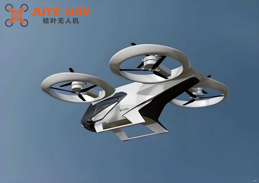
The following figure illustrates the typical structure and coordinate systems used for modeling a quadrotor drone. The inertial frame Oxyz is fixed to the ground, while the body-fixed frame O1x1y1z1 is attached to the vehicle’s center of mass. The control inputs are the thrust forces generated by the four rotors, which are combined to produce a total thrust and three body-axis moments.
Preliminary Concepts and Mathematical Model
1.1 Definitions and Lemmas
To facilitate the subsequent controller design and stability analysis, key concepts of finite-time stability and homogeneity are introduced.
Definition 1 (Homogeneity): Consider a nonlinear system:
$$\dot{\mathbf{x}} = \mathbf{f}(\mathbf{x}), \quad \mathbf{f}(\mathbf{0}) = \mathbf{0}, \quad \mathbf{x} \in \mathbb{R}^n$$
where $\mathbf{f}: U_0 \rightarrow \mathbb{R}^n$ is continuous on an open neighborhood $U_0$ of the origin. The vector field $\mathbf{f}(\mathbf{x}) = [f_1(\mathbf{x}), \ldots, f_n(\mathbf{x})]^T$ is said to be homogeneous of degree $k \in \mathbb{R}$ with respect to the dilation $(r_1, \ldots, r_n)$, where $r_i > 0$, if for any $\rho > 0$,
$$f_i(\rho^{r_1}x_1, \ldots, \rho^{r_n}x_n) = \rho^{k+r_i} f_i(x_1, \ldots, x_n), \quad i=1,\ldots,n.$$
If $\mathbf{f}$ is homogeneous, the system is called homogeneous.
Lemma 1: If the origin of a homogeneous system $\dot{\mathbf{x}} = \mathbf{f}(\mathbf{x})$ is asymptotically stable, then it is globally finite-time stable.
Lemma 2 (Finite-Time Stability): Consider the system $\dot{\mathbf{x}} = \mathbf{f}(\mathbf{x})$. If there exists a continuous positive definite function $V(\mathbf{x}): D \rightarrow \mathbb{R}$ such that
$$\dot{V}(\mathbf{x}) + c V^{\sigma}(\mathbf{x}) \leq 0, \quad \mathbf{x} \in D \setminus \{\mathbf{0}\}$$
where $c > 0$ and $\sigma \in (0,1)$, then the origin is a finite-time stable equilibrium. The settling time $T$ satisfies $T \leq V^{1-\sigma}(\mathbf{x}(0)) / [c(1-\sigma)]$.
We also define the function $\text{sig}^\alpha(x) = \text{sgn}(x)|x|^\alpha$ for scalar $x$, and $\text{sig}^\alpha(\mathbf{x}) = [\text{sig}^\alpha(x_1), \ldots, \text{sig}^\alpha(x_n)]^T$ for vector $\mathbf{x}$.
1.2 Dynamics of the Quadrotor Drone
The dynamic model of a quadrotor drone is derived using the Newton-Euler formalism. Let $\mathbf{r} = [x, y, z]^T$ denote the position in the inertial frame and $\boldsymbol{\Theta} = [\phi, \theta, \psi]^T$ represent the Euler angles (roll, pitch, yaw). The rotation matrix from the body frame to the inertial frame is $\mathbf{R}(\boldsymbol{\Theta})$. The translational dynamics are given by:
$$m\ddot{\mathbf{r}} = -mg\mathbf{e}_z + U \mathbf{R}(\boldsymbol{\Theta})\mathbf{e}_z + \mathbf{F}_A + \mathbf{F}_D,$$
where $m$ is the mass, $g$ is gravity, $U$ is the total thrust, $\mathbf{e}_z = [0,0,1]^T$, and $\mathbf{F}_A$, $\mathbf{F}_D$ are aerodynamic and external disturbance forces, respectively.
The rotational dynamics are:
$$\mathbf{J}\dot{\boldsymbol{\Omega}} = -\boldsymbol{\Omega} \times \mathbf{J}\boldsymbol{\Omega} + \boldsymbol{\tau} + \mathbf{M}_A + \mathbf{M}_D,$$
where $\mathbf{J}$ is the inertia tensor, $\boldsymbol{\Omega}$ is the angular velocity in the body frame, $\boldsymbol{\tau}$ is the control torque, and $\mathbf{M}_A$, $\mathbf{M}_D$ are aerodynamic and external disturbance moments. The kinematics relate $\dot{\boldsymbol{\Theta}}$ to $\boldsymbol{\Omega}$ via $\dot{\boldsymbol{\Theta}} = \mathbf{S}(\boldsymbol{\Theta})\boldsymbol{\Omega}$.
For controller design, these coupled equations can be decomposed into six single-input-single-output (SISO) channels by introducing virtual control inputs. The simplified dynamics for each channel $i$ ($i = x, y, z, \phi, \theta, \psi$) take the general form:
$$\ddot{\xi}_i = b_i u_i + f_i(t, \xi_i, \dot{\xi}_i) + w_i(t),$$
where $\xi_i$ is the output (position or attitude), $u_i$ is the virtual control input, $b_i$ is a known input gain, $f_i(\cdot)$ encapsulates unmodeled dynamics and nonlinear coupling terms, and $w_i(t)$ is an external disturbance. The term $L_i(t) = f_i(\cdot) + w_i(t)$ is defined as the “generalized disturbance” or “total disturbance” for that channel.
Assumption 1: For any feasible motion of the quadrotor drone, the generalized disturbance $L_i(t)$ and its first-time derivative are bounded, i.e., $|L_i(t)| \leq M_{0i}$ and $|\dot{L}_i(t)| \leq M_{1i}$.
Finite-Time Convergent Extended State Observer (FTCESO)
To address the challenge of unmeasured states and unknown disturbances in each SISO channel of the quadrotor drone, a Finite-Time Convergent Extended State Observer is proposed.
Consider a second-order SISO system in the form:
$$\begin{aligned}
\dot{x}_1 &= x_2, \\
\dot{x}_2 &= f(t, x_1, x_2) + b u + w(t) = L(t) + b u, \\
y &= x_1,
\end{aligned}$$
where $x_2$ is not measured, $f(\cdot)$ is unknown, $w(t)$ is a disturbance, and $L(t)$ is the generalized disturbance satisfying Assumption 1. By defining an extended state $x_3 = L(t)$, the system is augmented as:
$$\begin{aligned}
\dot{x}_1 &= x_2, \\
\dot{x}_2 &= x_3 + b u, \\
\dot{x}_3 &= \dot{L}(t).
\end{aligned}$$
The proposed FTCESO for this augmented system is:
$$\begin{aligned}
\dot{\hat{x}}_1 &= \hat{x}_2 – k_1 \text{sig}^{\alpha}(\hat{x}_1 – y), \\
\dot{\hat{x}}_2 &= \hat{x}_3 – k_2 \text{sig}^{\alpha}(\hat{x}_1 – y) + b u, \\
\dot{\hat{x}}_3 &= – k_3 \text{sig}^{\alpha}(\hat{x}_1 – y),
\end{aligned}$$
where $\hat{x}_1$, $\hat{x}_2$, $\hat{x}_3$ are the estimates of $x_1$, $x_2$, $x_3$ respectively, $k_1, k_2, k_3 > 0$ are observer gains, and $\alpha \in (0,1)$ is a design parameter. The $\text{sig}^{\alpha}(\cdot)$ function introduces a nonlinear correction term that enables finite-time convergence.
2.1 Stability Analysis of the FTCESO
Define the estimation errors as $\varepsilon_1 = \hat{x}_1 – x_1$, $\varepsilon_2 = \hat{x}_2 – x_2$, $\varepsilon_3 = \hat{x}_3 – x_3$. The error dynamics are:
$$\begin{aligned}
\dot{\varepsilon}_1 &= \varepsilon_2 – k_1 \text{sig}^{\alpha}(\varepsilon_1), \\
\dot{\varepsilon}_2 &= \varepsilon_3 – k_2 \text{sig}^{\alpha}(\varepsilon_1), \\
\dot{\varepsilon}_3 &= – k_3 \text{sig}^{\alpha}(\varepsilon_1) – \dot{L}(t).
\end{aligned}$$
Let $\boldsymbol{\eta} = [\text{sig}^{\alpha+1}(\varepsilon_1), \varepsilon_2, \varepsilon_3]^T$. The following theorem establishes the finite-time convergence of the observer.
Theorem 1: For the FTCESO applied to system, if Assumption 1 holds, then there exist gains $k_1, k_2, k_3 > 0$ and a finite time $t_s > 0$ such that the estimation error $\boldsymbol{\eta}$ converges to a small neighborhood of zero within $t_s$. Specifically, $||\boldsymbol{\eta}||$ enters the set $\{ \boldsymbol{\eta} : ||\boldsymbol{\eta}|| \leq l M_1 / [\sigma_{\text{min}}(\mathbf{A}) \sigma_{\text{min}}(\mathbf{P})] \}$ in finite time, where $l$ is a constant related to $k_3$, $M_1$ is the bound on $|\dot{L}(t)|$, $\mathbf{A}$ is a state-dependent matrix derived from the error dynamics, $\mathbf{P}$ is a positive definite matrix satisfying a Lyapunov equation, and $\sigma_{\text{min}}(\cdot)$ denotes the minimum singular value. By selecting sufficiently large gains, the ultimate bound on the estimation error can be made arbitrarily small.
Proof (Sketch): A candidate Lyapunov function $V(\boldsymbol{\eta}) = \boldsymbol{\eta}^T \mathbf{P} \boldsymbol{\eta}$ is constructed. Using the homogeneity properties of the error dynamics and Lemma 2, it can be shown that $\dot{V} \leq -C V^{1/2}$ holds after a finite time, guaranteeing finite-time convergence to a bounded region whose size is inversely proportional to the observer gains. This proves that $\hat{x}_1 \rightarrow x_1$, $\hat{x}_2 \rightarrow x_2$, and $\hat{x}_3 \rightarrow L(t)$ in finite time with bounded errors.
Composite Controller Design with FTCESO Compensation
With accurate estimates of both state and generalized disturbance provided by the FTCESO, a composite control law can be designed. The objective is to force the output $y=x_1$ to track a desired reference signal $y_r(t)$ with finite-time convergence properties.
Consider the tracking errors $e_1 = x_1 – y_r$ and $e_2 = x_2 – \dot{y}_r$. Using the estimates from the FTCESO, we define $\hat{e}_1 = \hat{x}_1 – y_r$ and $\hat{e}_2 = \hat{x}_2 – \dot{y}_r$.
Theorem 2: For the SISO system, if the control law is designed as:
$$u = \frac{1}{b} \left[ \ddot{y}_r – \hat{x}_3 – \kappa_1 \text{sig}^{\beta_1}(\hat{e}_1) – \kappa_2 \text{sig}^{\beta_2}(\hat{e}_2) \right],$$
where $\hat{x}_3$ is the disturbance estimate from the FTCESO, $\kappa_1, \kappa_2 > 0$, $\beta_1 \in (0,1)$, and $\beta_2 = 2\beta_1/(1+\beta_1)$, then the closed-loop tracking error dynamics are finite-time stable. The tracking error converges to a small neighborhood of zero in finite time.
Proof (Sketch): Substituting the control law into the original dynamics and using the estimation errors from the FTCESO leads to a perturbed error system:
$$\begin{aligned}
\dot{\tilde{e}}_1 &= \tilde{e}_2, \\
\dot{\tilde{e}}_2 &= -\kappa_1 \text{sig}^{\beta_1}(\tilde{e}_1 + \varepsilon_1) – \kappa_2 \text{sig}^{\beta_2}(\tilde{e}_2 + \varepsilon_2) + \Delta,
\end{aligned}$$
where $\tilde{e}_i$ are filtered errors, $\varepsilon_i$ are the bounded FTCESO estimation errors, and $\Delta$ is a bounded perturbation term. The nominal system (with $\varepsilon_i=0, \Delta=0$) is homogeneous and can be shown to be globally finite-time stable via a Lyapunov analysis. Using the boundedness of the perturbations from Theorem 1, the overall system is practically finite-time stable, meaning errors converge to a small residual set in finite time.
This composite strategy actively compensates for the generalized disturbance $\hat{x}_3$, significantly enhancing robustness. When $\beta_1=1$, the controller simplifies to a disturbance-compensated PD controller.
Application to Quadrotor Drone Control
The control of the quadrotor drone is separated into an outer-loop trajectory tracking controller and an inner-loop attitude stabilizing controller, both following the FTCESO-based composite design principle.
3.1 Trajectory Tracking Control
The translational dynamics can be rewritten as:
$$\ddot{\mathbf{r}} = \frac{1}{m} \mathbf{u} + \boldsymbol{\Gamma}_r(t),$$
where $\mathbf{u} = [u_x, u_y, u_z]^T$ is a virtual control vector defined by $\mathbf{u} = U \mathbf{R}(\boldsymbol{\Theta})\mathbf{e}_z$, and $\boldsymbol{\Gamma}_r(t)$ aggregates all other terms (gravity, aerodynamics, disturbances) as a generalized disturbance vector. Three independent FTCESOs are designed for the $x$, $y$, and $z$ channels as per Eq. (FTCESO), with outputs $r_x, r_y, r_z$ and inputs $u_x/m, u_y/m, u_z/m$.
Let $\mathbf{e}_r = \hat{\boldsymbol{\eta}}_1 – \mathbf{r}_c$ and $\dot{\mathbf{e}}_r = \hat{\boldsymbol{\eta}}_2 – \dot{\mathbf{r}}_c$, where $\hat{\boldsymbol{\eta}}_1$, $\hat{\boldsymbol{\eta}}_2$, $\hat{\boldsymbol{\Gamma}}_r$ are the FTCESO estimates for position, velocity, and disturbance. The virtual control law is:
$$\mathbf{u} = m \left[ \ddot{\mathbf{r}}_c – \hat{\boldsymbol{\Gamma}}_r – \mathbf{K}_{r1} \text{sig}^{\beta_1}(\mathbf{e}_r) – \mathbf{K}_{r2} \text{sig}^{\beta_2}(\dot{\mathbf{e}}_r) \right],$$
where $\mathbf{K}_{r1}, \mathbf{K}_{r2}$ are positive definite diagonal gain matrices. The total thrust $U$ and desired attitude angles $\phi_c, \theta_c$ are then derived from $\mathbf{u}$:
$$U = ||\mathbf{u}||, \quad \theta_c = \arctan\left( \frac{u_x \cos\psi_c + u_y \sin\psi_c}{u_z + g} \right), \quad \phi_c = \arcsin\left( \frac{u_x \sin\psi_c – u_y \cos\psi_c}{U} \right).$$
The yaw angle $\psi_c$ is independently specified.
3.2 Attitude Stabilization Control
Similarly, the rotational dynamics are expressed as:
$$\ddot{\boldsymbol{\Theta}} = \mathbf{J}^{-1} \boldsymbol{\tau} + \boldsymbol{\Gamma}_{\Theta}(t),$$
where $\boldsymbol{\Gamma}_{\Theta}(t)$ is the generalized disturbance for the attitude loop. Three FTCESOs are designed for the $\phi$, $\theta$, and $\psi$ channels. The control torque is computed as:
$$\boldsymbol{\tau} = \mathbf{J} \left[ \ddot{\boldsymbol{\Theta}}_c – \hat{\boldsymbol{\Gamma}}_{\Theta} – \mathbf{K}_{\Theta 1} \text{sig}^{\beta_1}(\mathbf{e}_{\Theta}) – \mathbf{K}_{\Theta 2} \text{sig}^{\beta_2}(\dot{\mathbf{e}}_{\Theta}) \right],$$
where $\mathbf{e}_{\Theta} = \hat{\boldsymbol{\zeta}}_1 – \boldsymbol{\Theta}_c$, $\dot{\mathbf{e}}_{\Theta} = \hat{\boldsymbol{\zeta}}_2 – \dot{\boldsymbol{\Theta}}_c$, and $\hat{\boldsymbol{\zeta}}_1, \hat{\boldsymbol{\zeta}}_2, \hat{\boldsymbol{\Gamma}}_{\Theta}$ are the attitude FTCESO estimates.
The overall control structure for the quadrotor drone is highly modular, with identical FTCESO and controller architectures for all six degrees of freedom, simplifying implementation and tuning. The key parameters for the FTCESO and the controllers are summarized below.
| Component | Parameter | Value / Setting |
|---|---|---|
| FTCESO (All Channels) | Gains $k_1, k_2, k_3$ | 25, 840, 950 |
| Nonlinear Exponent $\alpha$ | 0.4 | |
| Convergence Property | Finite-Time Practical Convergence | |
| Estimated Quantities | State ($\hat{x}_1$, $\hat{x}_2$) and Total Disturbance ($\hat{x}_3$) | |
| Trajectory Controller | Gain Matrices $\mathbf{K}_{r1}, \mathbf{K}_{r2}$ | $\text{diag}(200,200,200)$, $\text{diag}(100,100,100)$ |
| Exponents $\beta_1, \beta_2$ | 0.7, $2\beta_1/(1+\beta_1) \approx 0.82$ | |
| Thrust Saturation $U_{\text{max}}$ | 12 N | |
| Attitude Controller | Gain Matrices $\mathbf{K}_{\Theta 1}, \mathbf{K}_{\Theta 2}$ | $\text{diag}(200,200,200)$, $\text{diag}(40,40,40)$ |
| Exponents $\beta_1, \beta_2$ | 0.7, $2\beta_1/(1+\beta_1) \approx 0.82$ |
Simulation Results and Analysis
To validate the proposed FTCESO-based control framework for the quadrotor drone, comprehensive numerical simulations were conducted under challenging conditions, including parameter uncertainties, unmodeled aerodynamics, and sustained/time-varying external disturbances. The simulation model uses the full dynamics with a 4th-order Runge-Kutta solver (step size 0.005 s). The nominal physical parameters of the quadrotor drone are listed below.
| Parameter | Symbol | Value | Unit |
|---|---|---|---|
| Mass | $m$ | 0.74 | kg |
| Gravity | $g$ | 9.81 | m/s² |
| Arm Length | $l$ | 0.21 | m |
| Moment of Inertia (x/y/z) | $J_x, J_y, J_z$ | 0.0040, 0.0040, 0.0084 | kg·m² |
| Drag Coefficients | $C_{Dx}, C_{Dy}, C_{Dz}$ | 0.30, 0.30, 0.30 | – |
| Damping Coefficients | $C_{D\phi}, C_{D\theta}, C_{D\psi}$ | 0.01, 0.01, 0.01 | N·m·s/rad |
Robustness is tested with ±30% variations in mass $m$ and inertias $J_x, J_y, J_z$. Significant external disturbances are injected at different times: sinusoidal force disturbances on the x and y axes ($A_x, A_y$), a step plus sinusoidal force on the z-axis ($A_z$), and step plus sinusoidal moment disturbances on all three attitude axes ($M_\phi, M_\theta, M_\psi$).
The desired trajectory is a 3D Lissajous-like path: $x_r(t)=0.5\cos(\pi t/20)$, $y_r(t)=0.5\sin(\pi t/20)$, $z_r(t)=2-0.5\cos(\pi t/20)$, with $\psi_r(t)=0$ rad.
The simulation results demonstrate the effectiveness of the controller. The quadrotor drone successfully tracks the reference trajectory in 3D space under both nominal and perturbed conditions. Position tracking errors converge rapidly to near zero and remain small despite the applied disturbances. The attitude controller accurately tracks the angles commanded by the outer loop ($\phi_c, \theta_c$), with errors generally below 0.2 rad. The control inputs (total thrust $U$ and torques $\tau_\phi, \tau_\theta, \tau_\psi$) remain within feasible limits throughout the flight, confirming the practical viability of the approach. The FTCESOs effectively reconstruct and compensate for the generalized disturbances, which is key to maintaining performance amidst uncertainties.
Conclusion
This article has presented a robust control solution for a quadrotor drone by integrating Finite-Time Convergent Extended State Observers with a homogeneous feedback control law. The core of the method lies in treating complex, coupled nonlinearities and external influences as a generalized disturbance for each decoupled control channel. The proposed FTCESO provides accurate, finite-time estimates of both system states and this total disturbance using only output measurements. These estimates are then actively canceled in the control law, leading to a composite controller that is highly robust. The framework was systematically applied to both the translational and rotational dynamics of the quadrotor drone. Simulation studies under severe parameter uncertainties and external disturbances confirm that the proposed strategy ensures precise trajectory tracking and attitude stabilization. The control performance degrades minimally in the face of significant unmodeled effects, demonstrating the practical strength and disturbance rejection capability of the FTCESO-based approach for autonomous flight of quadrotor drones.