
The quadrotor drone has cemented its position as a pivotal platform in both civilian and military domains. Its advantages, including relatively low cost, mechanical simplicity, vertical take-off and landing (VTOL) capability, and hovering agility, make it ideal for applications ranging from aerial photography and precision agriculture to infrastructure inspection and search-and-rescue operations. However, the flight control problem for a quadrotor drone remains a significant challenge due to the system’s inherent characteristics: it is underactuated, highly nonlinear, and strongly coupled. With only four independent motor inputs, the vehicle must control six degrees of freedom (three translational and three rotational), leading to its underactuated nature. Furthermore, the rotational dynamics are coupled with translational motion through trigonometric functions, and gyroscopic effects introduce additional coupling between axes.
Traditional linear control methods, such as Proportional-Integral-Derivative (PID) controllers, are widely used due to their simplicity but often struggle to provide optimal performance across the entire flight envelope, especially during aggressive maneuvers or in the presence of significant disturbances. This has driven extensive research into more advanced control strategies. Among these, Model Predictive Control (MPC) has emerged as a powerful framework. MPC’s core strength lies in its ability to explicitly handle state and input constraints while optimizing control actions over a finite prediction horizon based on a dynamic model of the system. This makes it exceptionally well-suited for the trajectory tracking problem of a quadrotor drone, where actuator limits and safety boundaries must be rigorously respected.
This article presents a comprehensive review and technical exposition of a dual-loop MPC-based control architecture for quadrotor drone trajectory tracking. We begin by deriving the nonlinear dynamic model. Subsequently, we detail the cascaded control structure: an outer loop MPC for position/velocity control and an inner loop MPC, formulated for a Linear Parameter-Varying (LPV) representation of the attitude dynamics, for precise angular control. We will also situate this approach within the broader landscape of contemporary control strategies for quadrotor drones.
Nonlinear Dynamic Modeling of the Quadrotor Drone
To design any model-based controller, an accurate dynamic model is essential. We make the standard assumptions: the quadrotor drone is a rigid body with symmetrical structure and constant mass; the earth-fixed inertial frame is defined by axes \(\{X_E, Y_E, Z_E\}\) with \(Z_E\) pointing upwards; and the body-fixed frame is attached to the center of mass with axes \(\{X_B, Y_B, Z_B\}\).
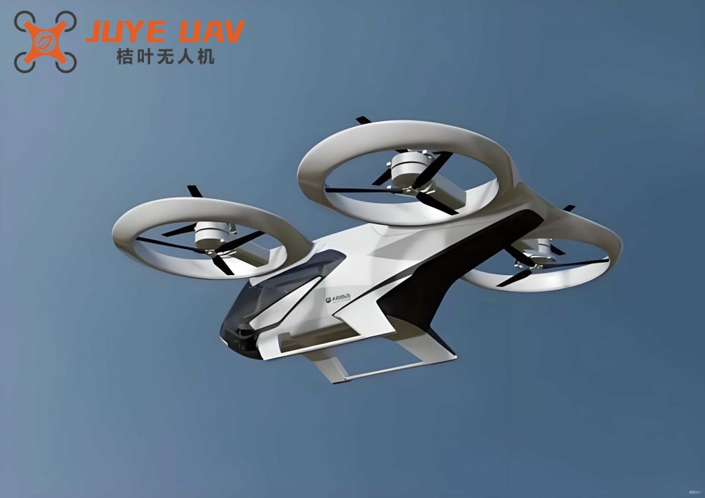
The vehicle’s pose is defined by its position \(\boldsymbol{\zeta} = [x, y, z]^T\) in the inertial frame and its orientation, represented by the Z-Y-X Euler angles \(\boldsymbol{\eta} = [\phi, \theta, \psi]^T\) (roll, pitch, yaw). The body angular rates are \(\boldsymbol{\omega}_B = [p, q, r]^T\). The Newton-Euler formalism yields the following equations of motion:
$$ m \ddot{\boldsymbol{\zeta}} = \boldsymbol{F} $$
$$ \boldsymbol{I} \dot{\boldsymbol{\omega}}_B = -\boldsymbol{\omega}_B \times (\boldsymbol{I} \boldsymbol{\omega}_B) + \boldsymbol{\tau} – \boldsymbol{\tau}_g $$
Here, \(m\) is the mass, \(\boldsymbol{I} = \text{diag}(I_{xx}, I_{yy}, I_{zz})\) is the inertia matrix, \(\boldsymbol{F}\) is the total external force vector in the inertial frame, \(\boldsymbol{\tau}\) is the total external torque vector in the body frame, and \(\boldsymbol{\tau}_g\) represents gyroscopic torques from the rotors.
The primary forces and moments are generated by the four rotors. Each rotor produces a thrust \(F_i = k_f \omega_i^2\) and a reactive torque \(M_i = k_m \omega_i^2\), where \(\omega_i\) is the rotational speed of the \(i\)-th motor, \(k_f\) is the thrust coefficient, and \(k_m\) is the torque coefficient. The control inputs for a standard quadrotor drone configuration are derived from combinations of these rotor speeds:
$$
\begin{aligned}
U_1 &= F_1 + F_2 + F_3 + F_4 = k_f (\omega_1^2 + \omega_2^2 + \omega_3^2 + \omega_4^2) \\
U_2 &= l (F_4 – F_2) = k_f l (\omega_4^2 – \omega_2^2) \\
U_3 &= l (F_3 – F_1) = k_f l (\omega_3^2 – \omega_1^2) \\
U_4 &= M_1 – M_2 + M_3 – M_4 = k_m (\omega_1^2 – \omega_2^2 + \omega_3^2 – \omega_4^2)
\end{aligned}
$$
where \(l\) is the arm length from the center of mass to each rotor. \(U_1\) is the total thrust force (along \(Z_B\)), \(U_2\) and \(U_3\) are the rolling and pitching moments, and \(U_4\) is the yawing moment.
The total force in the inertial frame is the sum of the rotated thrust vector and gravity: \(\boldsymbol{F} = \boldsymbol{R}(\phi, \theta, \psi) \cdot [0, 0, U_1]^T + [0, 0, -mg]^T\), where \(\boldsymbol{R}\) is the rotation matrix from body to inertial frame. Assuming small gyroscopic effects are negligible (\(\boldsymbol{\tau}_g \approx 0\)), the complete nonlinear dynamics of the quadrotor drone can be written as:
$$
\begin{aligned}
\ddot{x} &= (\cos\psi\sin\theta\cos\phi + \sin\psi\sin\phi)\frac{U_1}{m} \\
\ddot{y} &= (\sin\psi\sin\theta\cos\phi – \cos\psi\sin\phi)\frac{U_1}{m} \\
\ddot{z} &= (\cos\theta\cos\phi)\frac{U_1}{m} – g \\
\ddot{\phi} &= \dot{\theta}\dot{\psi} \left( \frac{I_{yy} – I_{zz}}{I_{xx}} \right) + \frac{U_2}{I_{xx}} \\
\ddot{\theta} &= \dot{\phi}\dot{\psi} \left( \frac{I_{zz} – I_{xx}}{I_{yy}} \right) + \frac{U_3}{I_{yy}} \\
\ddot{\psi} &= \dot{\phi}\dot{\theta} \left( \frac{I_{xx} – I_{yy}}{I_{zz}} \right) + \frac{U_4}{I_{zz}}
\end{aligned}
$$
This model clearly exhibits the underactuation and nonlinear coupling. The translational accelerations \((\ddot{x}, \ddot{y}, \ddot{z})\) depend nonlinearly on all three Euler angles and the single input \(U_1\), while the rotational dynamics are coupled through the products of angular rates.
Fundamentals of Model Predictive Control (MPC)
Model Predictive Control is an advanced control strategy that uses an explicit model of the plant to predict its future behavior over a finite horizon \(N_p\). At each sampling instant \(k\), it solves an online optimization problem to determine a sequence of control moves \(\{\boldsymbol{u}(k|k), \boldsymbol{u}(k+1|k), …, \boldsymbol{u}(k+N_c-1|k)\}\) that minimizes a cost function, typically penalizing tracking error and control effort, subject to system constraints. Only the first control move \(\boldsymbol{u}(k|k)\) is applied to the plant. At the next step, the horizon shifts forward, and the optimization is repeated with updated state measurements, making it a receding horizon strategy.
For a discrete-time state-space model \(\boldsymbol{x}(k+1) = \boldsymbol{A} \boldsymbol{x}(k) + \boldsymbol{B} \boldsymbol{u}(k)\), the standard quadratic MPC problem is:
$$
\begin{aligned}
\min_{\boldsymbol{U}_k} \quad & J(k) = \sum_{j=1}^{N_p} \|\boldsymbol{x}(k+j|k) – \boldsymbol{x}_{ref}(k+j)\|_{\boldsymbol{Q}}^2 + \sum_{j=0}^{N_c-1} \|\boldsymbol{u}(k+j|k) – \boldsymbol{u}_{ref}(k+j)\|_{\boldsymbol{R}}^2 \\
\text{subject to:} \quad & \boldsymbol{x}(k+j+1|k) = \boldsymbol{A} \boldsymbol{x}(k+j|k) + \boldsymbol{B} \boldsymbol{u}(k+j|k) \\
& \boldsymbol{u}_{min} \leq \boldsymbol{u}(k+j|k) \leq \boldsymbol{u}_{max} \\
& \boldsymbol{x}_{min} \leq \boldsymbol{x}(k+j|k) \leq \boldsymbol{x}_{max}
\end{aligned}
$$
where \(\boldsymbol{U}_k = [\boldsymbol{u}(k|k)^T, …, \boldsymbol{u}(k+N_c-1|k)^T]^T\), \(\boldsymbol{Q} \succeq 0\) and \(\boldsymbol{R} \succ 0\) are weighting matrices, and \(N_c \leq N_p\) is the control horizon. For linear models with quadratic cost and linear constraints, this problem reduces to a Quadratic Program (QP), which can be solved efficiently.
Dual-Loop MPC Architecture for Quadrotor Drone Control
A single, centralized MPC controller for the full 6-DOF nonlinear quadrotor drone model leads to a complex, high-dimensional, and nonlinear optimization problem that may be computationally prohibitive for real-time implementation on typical onboard hardware. A practical and effective alternative is the cascaded (dual-loop) control structure.
This architecture decomposes the problem into two layers:
- Outer Loop (Position/Velocity Control): This loop takes the desired trajectory \(\boldsymbol{\zeta}_{ref}(t), \dot{\boldsymbol{\zeta}}_{ref}(t)\) as input and computes the required total thrust \(U_1\) and desired attitude angles \((\phi_d, \theta_d, \psi_d)\).
- Inner Loop (Attitude Control): This loop receives the desired attitude from the outer loop and computes the required moments \(U_2, U_3, U_4\) to track it rapidly.
The key idea is that the inner-loop attitude controller operates at a much higher bandwidth than the outer-loop position controller, allowing the assumption that the attitude can be controlled to its desired value almost instantaneously from the perspective of the slower outer loop.
Outer Loop: MPC for Position and Velocity Tracking
We define the outer-loop state vector as \(\boldsymbol{x}_o = [x, \dot{x}, y, \dot{y}, z, \dot{z}]^T\) and the virtual control input as \(\boldsymbol{v} = [a_x, a_y, a_z]^T\), where \(a_x, a_y, a_z\) are the desired accelerations in the inertial frame. From the translational dynamics, we have \(\ddot{x} = a_x\), \(\ddot{y} = a_y\), \(\ddot{z} = a_z – g\). Discretizing this double-integrator model with sample time \(T_s\) yields a linear time-invariant (LTI) state-space model suitable for MPC:
$$ \boldsymbol{x}_o(k+1) = \boldsymbol{A}_o \boldsymbol{x}_o(k) + \boldsymbol{B}_o \boldsymbol{v}(k) $$
where
$$
\boldsymbol{A}_o = \text{blkdiag}(\boldsymbol{A}_{1D}, \boldsymbol{A}_{1D}, \boldsymbol{A}_{1D}), \quad \boldsymbol{B}_o = \text{blkdiag}(\boldsymbol{B}_{1D}, \boldsymbol{B}_{1D}, \boldsymbol{B}_{1D})
$$
with
$$ \boldsymbol{A}_{1D} = \begin{bmatrix} 1 & T_s \\ 0 & 1 \end{bmatrix}, \quad \boldsymbol{B}_{1D} = \begin{bmatrix} \frac{T_s^2}{2} \\ T_s \end{bmatrix}. $$
The MPC controller for the outer loop solves the QP problem at each step to find the optimal sequence of accelerations \(\boldsymbol{V}_k\). The first optimal acceleration \(\boldsymbol{v}^*(k|k) = [a_x^*, a_y^*, a_z^*]^T\) is then converted into physical control commands for the quadrotor drone. First, the required total thrust is:
$$ U_1 = m \cdot \| [a_x^*, a_y^*, a_z^* + g]^T \|. $$
Assuming the yaw angle \(\psi_d\) is independently specified (often set to zero or a constant for many tasks), the desired roll and pitch angles are derived by inverting the translational dynamics relationship:
$$
\begin{aligned}
\phi_d &= \arcsin\left( m \frac{a_x^* \sin\psi_d – a_y^* \cos\psi_d}{U_1} \right) \\
\theta_d &= \arctan\left( \frac{a_x^* \cos\psi_d + a_y^* \sin\psi_d}{a_z^* + g} \right)
\end{aligned}
$$
These desired angles \((\phi_d, \theta_d, \psi_d)\) are passed to the inner-loop attitude controller.
Inner Loop: LPV-MPC for Attitude Tracking
The inner-loop must track the desired attitude angles quickly and accurately. The attitude dynamics are nonlinear (see equations for \(\ddot{\phi}, \ddot{\theta}, \ddot{\psi}\)). Direct nonlinear MPC is possible but can be computationally heavy. An effective approach is to exploit the structure of the equations by representing them as a Linear Parameter-Varying (LPV) system. The state vector is \(\boldsymbol{x}_i = [\phi, \dot{\phi}, \theta, \dot{\theta}, \psi, \dot{\psi}]^T\) and the input is \(\boldsymbol{u}_i = [U_2, U_3, U_4]^T\).
We can rewrite the rotational dynamics as:
$$
\dot{\boldsymbol{x}}_i = \boldsymbol{A}_i(\boldsymbol{\rho}(t)) \boldsymbol{x}_i + \boldsymbol{B}_i \boldsymbol{u}_i
$$
where the system matrix \(\boldsymbol{A}_i\) depends on the scheduling parameters \(\boldsymbol{\rho}(t)\), which are measurable or estimated online. For the quadrotor drone, a common LPV formulation uses the angular rates as scheduling parameters:
$$
\boldsymbol{A}_i(\boldsymbol{\rho}) =
\begin{bmatrix}
0 & 1 & 0 & 0 & 0 & 0 \\
0 & 0 & 0 & \rho_1 & 0 & \rho_2 \\
0 & 0 & 0 & 1 & 0 & 0 \\
0 & \rho_3 & 0 & 0 & 0 & \rho_4 \\
0 & 0 & 0 & 0 & 0 & 1 \\
0 & \rho_5 & 0 & \rho_6 & 0 & 0
\end{bmatrix}, \quad
\boldsymbol{B}_i =
\begin{bmatrix}
0 & 0 & 0 \\
\frac{1}{I_{xx}} & 0 & 0 \\
0 & 0 & 0 \\
0 & \frac{1}{I_{yy}} & 0 \\
0 & 0 & 0 \\
0 & 0 & \frac{1}{I_{zz}}
\end{bmatrix}
$$
with
$$
\begin{aligned}
\rho_1 &= -\frac{I_p \omega_T}{I_{xx}}, & \rho_2 &= \dot{\theta} \frac{I_{yy}-I_{zz}}{I_{xx}}, \\
\rho_3 &= \frac{I_p \omega_T}{I_{yy}}, & \rho_4 &= \dot{\phi} \frac{I_{zz}-I_{xx}}{I_{yy}}, \\
\rho_5 &= \frac{\dot{\theta}}{2} \frac{I_{xx}-I_{yy}}{I_{zz}}, & \rho_6 &= \frac{\dot{\phi}}{2} \frac{I_{xx}-I_{yy}}{I_{zz}}.
\end{aligned}
$$
In this LPV-MPC formulation, at each sampling instant, the parameters \(\boldsymbol{\rho}(k)\) are frozen using the current state estimates (e.g., \(\dot{\phi}(k), \dot{\theta}(k)\)). The resulting time-varying linear model \(\boldsymbol{A}_i(k), \boldsymbol{B}_i\) is then used to construct the prediction matrices for the QP solver. This approach captures the main nonlinearities while maintaining a convex quadratic optimization problem. The inner-loop MPC solves:
$$
\begin{aligned}
\min_{\boldsymbol{U}_{i,k}} \quad & \sum_{j=1}^{N_p^i} \|\boldsymbol{x}_i(k+j|k) – \boldsymbol{x}_{i,ref}(k+j)\|_{\boldsymbol{Q}_i}^2 + \sum_{j=0}^{N_c^i-1} \|\boldsymbol{u}_i(k+j|k)\|_{\boldsymbol{R}_i}^2 \\
\text{s.t.} \quad & \text{LPV prediction model with } \boldsymbol{\rho}(k), \\
& \boldsymbol{u}_{i,min} \leq \boldsymbol{u}_i(k+j|k) \leq \boldsymbol{u}_{i,max}
\end{aligned}
$$
where \(\boldsymbol{x}_{i,ref} = [\phi_d, 0, \theta_d, 0, \psi_d, 0]^T\). The solution provides the optimal moments \(U_2^*, U_3^*, U_4^*\) to be applied to the quadrotor drone.
Comparison with Other Advanced Control Strategies
While dual-loop MPC presents a robust framework, the field of quadrotor drone control is rich with alternative and complementary approaches. The table below summarizes several key methodologies.
| Control Strategy | Core Principle | Advantages for Quadrotor Drone | Challenges/Limitations |
|---|---|---|---|
| Cascaded PID | Multiple single-input-single-output PID loops in a hierarchical structure. | Extremely simple, easy to tune and implement, widely used in commercial platforms. | Poor handling of coupling and nonlinearities; performance degrades during aggressive maneuvers. |
| Linear Quadratic Regulator (LQR) | Optimal state feedback for a linearized model minimizing a quadratic cost. | Provides optimal gains for the linearized point; good performance near hover. | Performance away from the linearization point is not guaranteed; cannot handle constraints directly. |
| Feedback Linearization | Uses nonlinear state feedback to transform the system into a linear one. | Can theoretically achieve global linearization and decoupling. | Relies on exact model knowledge; sensitive to model uncertainties and disturbances; control inputs can become large. |
| Sliding Mode Control (SMC) | Forces system trajectories to slide along a predefined surface, robust to matched uncertainties. | High robustness to disturbances and model variations. | Inherent chattering phenomenon, which can excite unmodeled dynamics and wear actuators. |
| Active Disturbance Rejection Control (ADRC) | Estimates and cancels total disturbances (internal dynamics + external forces) via an Extended State Observer (ESO). | Very effective in dealing with unmodeled dynamics and external gusts; model-light approach. | Observer bandwidth and noise sensitivity require careful tuning; stability proofs can be complex. |
| Robust Control (e.g., H∞) | Optimizes controller to minimize worst-case effect of disturbances/uncertainties. | Provides guaranteed performance and stability margins under bounded uncertainties. | Design can be conservative; resulting controllers may be of high order. |
| Learning-Based Control (e.g., RL, Adaptive) | Uses data to adapt controller parameters or learn control policy directly. | Can adapt to changing dynamics or poorly modeled effects; great potential for complex tasks. | Requires extensive data/training; safety and stability guarantees during learning are major concerns. |
| Dual-Loop MPC (This Article) | Uses model-based online optimization for constrained control in a cascaded structure. | Explicit constraint handling; optimal performance w.r.t. a cost function; natural for trajectory tracking. | Computational burden hinges on model complexity and horizon length; requires accurate real-time state estimation. |
A notable trend is the hybridization of these methods. For instance, MPC can be combined with disturbance observers (like ADRC’s ESO) to improve robustness. The paper cited in the initial prompt mentions using an Extended State Kalman Filter (ESKF) to estimate wind disturbances for an MPC, creating an ESKF-MPC scheme. Similarly, non-singular terminal sliding mode controllers can be used in the inner loop with fuzzy logic tuning for the outer loop, as explored in other research. These hybrid approaches aim to marry the strengths of different paradigms to create more capable controllers for the demanding quadrotor drone platform.
Simulation, Implementation, and Performance Analysis
Validating the dual-loop MPC architecture requires rigorous simulation before real-world deployment. The typical workflow involves the following steps:
- High-Fidelity Modeling: Implement the nonlinear dynamics in a simulation environment like MATLAB/Simulink, including realistic actuator models (saturation, rate limits) and sensor noise.
- Controller Discretization and Tuning: Discretize the MPC models for both loops with appropriate sample times (e.g., 50-100 ms for outer loop, 5-20 ms for inner loop). Tune the weighting matrices \(\boldsymbol{Q}, \boldsymbol{R}\) and prediction horizons \(N_p, N_c\) to achieve desired performance. A common tuning principle is to prioritize tracking in \(\boldsymbol{Q}\) while using \(\boldsymbol{R}\) to penalize aggressive control actions.
- QP Solver Integration: Employ an efficient QP solver (e.g., qpOASES, OSQP, or MATLAB’s
quadprog) to solve the optimization problem at each time step within the allocated sampling period. - Trajectory Generation: Define smooth, dynamically feasible reference trajectories for position and yaw. Common patterns include hovering set-points, lemniscates, sinusoidal waves, or complex 3D paths.
- State Estimation: In practice, a state estimator (e.g., Complementary Filter, Extended Kalman Filter) is crucial to provide accurate full-state feedback from onboard IMU and GPS/vision data. The estimator dynamics can also be included in the simulation.
Key performance metrics to evaluate the quadrotor drone controller include:
- Tracking Error: Root Mean Square Error (RMSE) and maximum absolute error for position \((x, y, z)\) and attitude \((\phi, \theta, \psi)\).
- Control Effort: Total variation and magnitude of control inputs \(U_1, U_2, U_3, U_4\).
- Robustness: Performance under model parameter uncertainties (e.g., +/- 20% mass/inertia error) and external disturbances (e.g., step wind gusts).
- Computational Timing: The maximum and average time required to solve the QP, which must be consistently less than the sampling time.
Simulation results from the described dual-loop MPC typically show excellent trajectory tracking with very small steady-state error, smooth control inputs that respect predefined constraints, and good rejection of moderate disturbances. The LPV-MPC inner loop is particularly effective at handling the nonlinear coupling during aggressive turns compared to a simple linear MPC based on a Jacobian linearization at hover.
Challenges and Future Research Directions
Despite the proven effectiveness of MPC for quadrotor drone control, several challenges persist, driving current research:
- Computational Complexity: Real-time implementation on low-power flight controllers remains the primary hurdle. Research focuses on explicit MPC (pre-computing the control law offline), using simpler models (e.g., error dynamics), and leveraging faster embedded QP solvers.
- Model Accuracy and Robustness: MPC performance is intrinsically tied to model fidelity. Future work integrates adaptive MPC or robust MPC (like Tube-MPC) to handle parametric uncertainties and bounded disturbances explicitly in the optimization.
- Nonlinear MPC (NMPC): While more computationally demanding, NMPC applied to the full model promises superior performance. Advances in real-time optimization algorithms (e.g., ACADO, GRAMPC) and the use of high-performance embedded computing are making this increasingly feasible for complex quadrotor drone missions.
- Learning-Enhanced MPC: A promising direction is to use machine learning (e.g., Gaussian Processes, Neural Networks) to learn the residual model mismatch online and improve prediction accuracy, leading to a hybrid model-based/model-free architecture.
- Multi-Agent Coordination: Extending MPC to formations of multiple quadrotor drones involves distributed or decentralized MPC strategies, where each agent solves its own problem while communicating limited information with neighbors to achieve collective goals.
In conclusion, the dual-loop MPC architecture, particularly with an LPV-based inner loop, provides a powerful and structured framework for controlling a quadrotor drone. It successfully balances performance optimality, explicit constraint satisfaction, and implementational practicality. As computational power increases and algorithms become more sophisticated, MPC-based strategies are poised to become the standard for high-performance, reliable, and autonomous flight control of quadrotor drones in increasingly complex and dynamic environments.