
The advancement of unmanned aerial vehicle (UAV) technology has profoundly transformed modern agriculture, with the agricultural drone becoming a cornerstone of precision plant protection. These systems offer remarkable advantages in operational efficiency, cost reduction, water conservation, and ease of deployment. The planning for such agricultural drone operations generally falls into two categories: coverage path planning, which generates a complete flying route over a field, and mission planning, which determines optimal breakpoints for the drone to return to a depot for battery swapping or chemical refilling. While existing research has addressed multi-drone task allocation and simple refueling strategies, a significant gap remains in optimizing single-drone mission plans that incorporate the critical aspect of variable-rate prescription spraying. Prescription spraying, where the agricultural drone adjusts its application rate based on spatially variable pest or nutrient maps, is essential for enhancing efficacy and minimizing environmental impact. The common practice of operating until a battery or tank limit is reached—the “maximum distance mode”—often leads to inefficient non-operational travel.
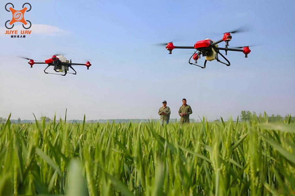
This article addresses this gap by presenting a novel mission planning methodology for a single agricultural drone performing prescription spraying. We establish a mathematical model that optimizes the return-to-depot points along a pre-computed coverage path. The model explicitly considers constraints from battery endurance and tank capacity under variable-rate application, with the dual objectives of minimizing total mission time and total non-operational travel distance. To solve this complex, non-linear optimization problem, we propose an Improved Spider Wasp Optimizer (ISWO). The ISWO enhances the original Spider Wasp Optimizer by integrating a sine-cosine adaptive contraction strategy with learning factors and a greedy-mean-based population initialization method. Extensive experimental analyses demonstrate that our ISWO-based planning method significantly outperforms the traditional maximum distance mode and shows superior optimization performance and stability compared to other established heuristic algorithms like WOA, GWO, PSO, and the original SWO.
Problem Definition and System Modeling
The core problem involves a single agricultural drone tasked with spraying a field along a pre-generated, boustrophedon (back-and-forth) coverage path. The drone starts from a depot, follows the path while spraying according to a prescription map, and must periodically interrupt its work to return to the depot for battery replacement and chemical refill. The point where it stops spraying to return is called a “return point.” The travel between the return point and the depot constitutes non-operational distance, which is pure overhead. The goal is to strategically plan the sequence of return points to minimize this overhead and the total mission time, while respecting the drone’s physical limits.
The workflow begins with generating a dense set of waypoints, \(\text{PATH} = \{p_1, p_2, …, p_n\}\), from the continuous coverage path. Each segment between waypoints \(p_{i-1}\) and \(p_i\) has associated properties: length \(l_i\), cumulative spray volume \(q_i\) (calculated based on the prescription value \(pr_i\) for that segment), and spatial coordinates. The depot location is denoted as \(P_b\).
The optimization model is built upon several key equations. The spray volume for a segment is calculated as:
$$q_i = \frac{l_i}{V} \times pr_i \times V_q$$
where \(V\) is the drone’s constant operating speed and \(V_q\) is the maximum flow rate of the spraying system. For a mission batch \(i\) (the work between two consecutive returns to the depot), the total chemical consumption \(Q_i\) and the battery energy consumption \(E_i\) are cumulative sums from the starting waypoint index \(S_{i-1}\) to the return point index \(S_i\). The non-operational distance \(O_i\) for batch \(i\) is the sum of the distances from the previous return point (or the start) to the depot and from the depot to the new return point:
$$O_i = \|P_{S_{i-1}} – P_b\| + \|P_{S_i} – P_b\|$$
A critical factor is the energy consumption ratio \(R_i\), which models the fact that a heavier drone (full tank) consumes more energy per unit distance than a lighter one (empty tank). It is defined as:
$$R_i = R_t + (1 – R_t) \times \frac{Q_i}{Q_{\text{max}}}$$
where \(R_t\) is the energy consumption ratio when the tank is empty relative to when it is full, and \(Q_{\text{max}}\) is the tank capacity. Consequently, the energy consumed in batch \(i\) includes the weighted operational distance and the weighted inbound/outbound travel:
$$E_i = \left( \sum_{j=S_{i-1}+1}^{S_i} l_j \right) \times R_i + \|P_{S_{i-1}} – P_b\| \times R_i + \|P_{S_i} – P_b\| \times R_t$$
The time for each batch \(F_i\) includes operational time, non-operational travel time, depot service time \(C_r\), and time for turns \(C_t \times C_i\):
$$F_i = \frac{1}{V} \sum_{j=S_{i-1}+1}^{S_i} l_j + \frac{O_i}{V_{\text{non}}} + C_r + C_t \times C_i$$
where \(V_{\text{non}}\) is the drone’s speed during non-operational travel.
The mission plan is defined by the set of return point indices, \(X = \{S_1, S_2, …, S_D\}\), where \(S_D = n\). This set is the decision variable for our optimization. Each plan must satisfy the hard constraints for every batch \(i\):
$$E_i \leq E_{\text{max}} \quad \text{(Battery Constraint)}$$
$$Q_i \leq Q_{\text{max}} \quad \text{(Tank Capacity Constraint)}$$
The objective function \(f\) to be minimized is the total mission time plus penalty terms for violating the constraints:
$$\min f = \sum_{i=1}^{D} F_i + \omega_1 E_o + \omega_2 Q_o$$
where \(E_o\) and \(Q_o\) are the normalized excess energy and chemical consumption beyond the limits \(E_{\text{max}}\) and \(Q_{\text{max}}\), and \(\omega_1, \omega_2\) are large penalty weights (e.g., ~1000) to strongly discourage infeasible solutions. When a solution is feasible, \(f\) equals the total mission time.
The Proposed Improved Spider Wasp Optimizer (ISWO)
Solving the model requires navigating a discrete, combinatorial search space with numerous local optima. We selected the Spider Wasp Optimizer (SWO) as a base due to its robust exploration-exploitation balance and strong ability to escape local optima. However, we introduce significant enhancements to tailor it to our specific problem, resulting in the ISWO.
The original SWO operates in four phases: Searching, Chasing, Nesting, and Mating. A spider wasp’s position represents a candidate solution (a set \(X\)). The update rules involve stochastic movements influenced by random peers, the global best, and specific patterns like Lévy flights.
Key Improvements in ISWO:
1. Modified Crossover Strategy: The Mating phase in SWO uses a standard crossover operator, which can break the strictly increasing order of the return point indices in \(X\). Our modified crossover ensures the last index remains fixed and sorts any pair of exchanged indices to maintain a valid sequence.
2. Adaptive Sine-Cosine Contraction Phase: The penalty-based objective creates a fitness landscape where feasible and infeasible solutions are separated by large values. To rapidly guide the population toward the feasible region early in the search, we introduce a new contraction phase. A particle updates its position using a mechanism inspired by the Sine Cosine Algorithm and PSO’s social/cognitive components:
$$
SW_i^{t+1} =
\begin{cases}
r_1 \cdot \cos(2\pi l) \cdot D’_G + r_2 \cdot \sin(2\pi l) \cdot D’_p + \lambda_1 SW_i^t + \lambda_2 SW^*_G + \lambda_3 SW^*_p, & r_4 < 0.5 \\
r_1 \cdot \sin(2\pi l) \cdot D’_G + r_2 \cdot \cos(2\pi l) \cdot D’_p + \lambda_1 SW_i^t + \lambda_2 SW^*_G + \lambda_3 SW^*_p, & r_4 \geq 0.5
\end{cases}
$$
where \(D’_G = |SW^*_G – SW_i^t| \cdot r_5\), \(D’_p = |SW^*_p – SW_i^t| \cdot r_5\). Here, \(SW^*_G\) is the best feasible solution in the swarm, \(SW^*_p\) is the particle’s personal best, and \(r_1\) to \(r_5\) and \(l\) are random numbers. The adaptive weights \(\lambda_1, \lambda_2, \lambda_3\) are dynamically calculated based on the fitness values of the three guiding solutions (\(SW_i^t, SW^*_p, SW^*_G\)), balancing their influence. This phase is controlled by an adaptive trigger probability \(TRR_t\) that is low initially to promote convergence to feasible areas and increases if stagnation is detected to switch back to SWO’s explorative phases.
3. Greedy-Mean Initialization: Instead of random initialization, we generate initial candidate solutions where the distances between consecutive return points are biased to be less than the drone’s effective range. This method produces a higher-quality initial population with more feasible individuals, accelerating convergence.
4. Solution Repair: Before evaluation, each candidate solution is repaired by ensuring the last point is the final waypoint and by adjusting return points that fall on turning segments to the next waypoint to avoid counting non-spraying turn distance as operational travel.
The overall algorithm flow is summarized in the following pseudocode structure:
Algorithm: ISWO for Agricultural Drone Mission Planning
1. Generate coverage path and waypoint set PATH.
2. Initialize population using Greedy-Mean method.
3. While stopping criterion not met do
4. For each spider wasp in population do
5. Apply Repair operator.
6. Evaluate fitness \(f\) (mission time + penalties).
7. Update personal best (\(SW^*_p\)).
8. End For
9. Update global best feasible solution (\(SW^*_G\)).
10. For each spider wasp do
11. If rand() < \(TRR_t\) then
12. Update position using Adaptive Sine-Cosine Contraction (Eq. above).
13. Else
14. Update position using standard SWO phases (Searching/Chasing/Nesting/Mating).
15. End If
16. End For
17. Adjust adaptive trigger \(TRR_t\) based on stagnation detection.
18. End While
19. If best solution has a batch with excessive remaining battery then
20. Reduce the number of returns \(D\) by 1 and re-optimize.
21. End If
22. Return the best mission plan \(X\).
Experimental Validation and Results Analysis
We conducted a series of simulation experiments to validate the effectiveness of our model and the performance of the ISWO algorithm. The simulation environment was configured with standard parameters for a typical agricultural drone.
| Parameter | Symbol | Value |
|---|---|---|
| Maximum Flow Rate | \(V_q\) | 0.04 L/s |
| Swath Width | \(d\) | 5 m |
| Operational Speed | \(V\) | 2.5 m/s |
| Non-Operational Speed | \(V_{\text{non}}\) | 2.5 m/s |
| Maximum Battery Endurance | \(E_{\text{max}}\) | 1500 m |
| Tank Capacity | \(Q_{\text{max}}\) | 10 L |
| Depot Service Time | \(C_r\) | 120 s |
| Turn Time | \(C_t\) | 10 s |
| Empty/Full Energy Ratio | \(R_t\) | 0.45 |
| Waypoint Sampling Interval | \(pl\) | 5 m |
Effectiveness Analysis vs. Maximum Distance Mode
We first compared the ISWO-planned mission against the traditional maximum distance mode on a 150m x 220m field with a prescription map. The maximum distance mode triggers a return when the battery reaches 30% remaining or the tank is empty.
| Metric | ISWO-Optimized Plan | Maximum Distance Mode | Improvement |
|---|---|---|---|
| Total Mission Time (s) | 4107 | 5646 | 27.3% reduction |
| Total Non-Operational Distance (m) | 606 | 1626 | 62.7% reduction |
| Number of Returns (D) | 6 | 7 | 1 less return |
The results are compelling. The ISWO algorithm strategically placed return points near the field boundary closest to the depot, drastically cutting down on deadhead travel. It also better utilized the drone’s capacity, allowing for longer operational stretches where efficient, leading to fewer total returns. This demonstrates the significant practical value of optimized mission planning for the agricultural drone.
Algorithm Performance and Scalability
To evaluate the optimization performance of ISWO, we compared it against the original SWO and other popular meta-heuristics: Whale Optimization Algorithm (WOA), Grey Wolf Optimizer (GWO), and Particle Swarm Optimization (PSO). Experiments were run on fields of increasing size. Each algorithm was executed 30 times per case to gather statistics on solution quality (best, mean fitness) and stability (standard deviation).
| Field Size | Algorithm | Best Fitness | Mean Fitness | Std. Dev. |
|---|---|---|---|---|
| 100m x 200m | WOA | 2421 | 2431 | 10.70 |
| GWO | 2421 | 2425 | 5.20 | |
| PSO | 2421 | 2427 | 7.25 | |
| SWO | 2421 | 2427 | 5.83 | |
| ISWO | 2421 | 2421.0 | 0.0 | |
| 220m x 300m | WOA | 8831 | 9099 | 168.09 |
| GWO | 9036 | 9491 | 143.29 | |
| PSO | 8871 | 9736 | 304.50 | |
| SWO | 8873 | 9134 | 98.50 | |
| ISWO | 8635 | 8740 | 42.86 |
ISWO consistently found the best or equal-best solutions across all tests. More importantly, it exhibited superior stability, evidenced by the lowest standard deviations, especially as problem complexity (field size and number of return points) increased. The adaptive contraction phase and smart initialization effectively guided the search, while the SWO backbone provided robust exploration. The convergence graphs clearly show ISWO reaching near-optimal regions much faster than the original SWO.
Parameter Sensitivity and Analysis
We investigated the sensitivity of ISWO to its key parameters. A full factorial analysis on the trigger probability for the standard SWO phases (\(TR\)) and the crossover rate (\(CR\)) showed that the algorithm is relatively robust, with stable performance across a range of values. Optimal stability was observed around \(TR=0.5\) and \(CR=0.4\).
The impact of the waypoint sampling interval \(pl\) is crucial. A finer sampling (smaller \(pl\)) increases the resolution of possible return points, potentially leading to better solutions but expanding the search space and computation time.
| Sampling \(pl\) (m) | Best Fitness (s) | Std. Dev. (s) | Avg. Runtime (s) |
|---|---|---|---|
| 2 | 6598 | 51.04 | 3.1 |
| 5 | 6616 | 23.45 | 2.5 |
| 10 | 6629 | 18.53 | 2.3 |
| 15 | 6727 | 7.40 | 1.87 |
As shown, a moderate \(pl\) (e.g., 5m or 10m) offers a good trade-off between solution quality, algorithm stability, and computational cost for the agricultural drone planning problem.
Conclusion and Future Work
This article presented a comprehensive solution for the mission planning of a single agricultural drone engaged in variable-rate prescription spraying. We formulated a realistic optimization model that minimizes total mission time and non-operational travel under battery and tank constraints. To solve this NP-hard problem, we proposed the Improved Spider Wasp Optimizer (ISWO), which incorporates an adaptive sine-cosine contraction strategy and a greedy initialization method to enhance convergence speed and solution quality.
Our experimental results demonstrate the practical necessity of such planning. Compared to the unplanned maximum distance mode, our method can reduce non-operational travel by over 60% and total mission time by nearly 30%. Furthermore, ISWO proved to be a more effective and stable solver for this problem than several state-of-the-art heuristic algorithms, making it a valuable tool for optimizing the operational efficiency of agricultural drone fleets.
Future research will focus on increasing the model’s fidelity. The current linear energy consumption model can be replaced with a more accurate, non-linear model derived from real-world flight data, accounting for variable load, altitude, wind, and acceleration during takeoff/landing. Integrating this planning module with real-time control systems and exploring robust planning under weather uncertainty are also promising directions for advancing the autonomy and reliability of agricultural drone operations.