
In modern agriculture, the use of agricultural drones for pesticide spraying has revolutionized crop protection by offering efficiency, precision, and reduced environmental impact. However, despite the advantages, applicators such as drone pilots and ground crew remain exposed to pesticides during operations, posing potential health risks. As a researcher focused on agricultural safety, I embarked on this study to evaluate the unit exposure levels across different body parts of applicators during agricultural drone applications. The goal is to leverage statistical and multi-criteria decision-making methods to provide data-driven recommendations for reducing exposure risks. This work emphasizes the importance of personalized safety protocols in the era of smart farming, where agricultural drones are becoming ubiquitous.
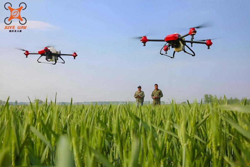
The adoption of agricultural drones has surged due to their ability to cover large areas quickly, minimize chemical drift, and reduce human labor in hazardous environments. Nonetheless, applicator exposure cannot be entirely eliminated, as highlighted in previous studies on traditional spray methods. For instance, manual backpack spraying often leads to significant exposure on the back and hands, whereas applications with agricultural drones may shift exposure patterns due to different operational dynamics. In this context, I designed a nested experiment to capture exposure variability across crops, applicator roles, and body parts. The primary objective is to identify body parts with the most controllable exposure, analyze correlations between exposures, and comprehensively rank applicators based on their risk profiles. By integrating Principal Component Analysis (PCA) and the Technique for Order Preference by Similarity to Ideal Solution (TOPSIS), this study aims to offer actionable insights for optimizing safety practices in agricultural drone operations.
The experiment employed a nested design with three factors. The first-level factor was the crop, with two levels: corn and rice. The second-level factor was the applicator role, including drone pilots and ground crew responsible for mixing and loading pesticides. The third-level factor involved 11 body parts of the protective clothing: head (MZ), neck (JB), upper arm (DB), forearm (XB), chest (QX), back (HB), thigh (DT), lower leg (XT), mask (KZ), gloves (ST), and feet (WZ). All applicators wore full protective gear during operations with an agricultural drone model similar to the DJI T16. The pesticide used was 25% chlorantraniliprole, with application rates of 270 g for rice and 300 g for corn, diluted to concentrations of 0.17 mL·L⁻¹ and 0.19 mL·L⁻¹, respectively. Environmental conditions during spraying included an average wind speed of 1.8 m·s⁻¹, relative humidity of 43%, and temperature of 26°C. After application, unit exposure levels (in µg·cm⁻²) were collected from each body part using whole-body sampling techniques, resulting in a dataset for 12 applicators.
To analyze the data, I applied several statistical methods. First, the coefficient of variation (CV) was calculated for each body part to assess the variability in exposure levels. The CV is defined as:
$$CV = \frac{\sigma}{\mu} \times 100\%$$
where $\sigma$ is the standard deviation and $\mu$ is the mean unit exposure. A higher CV indicates greater variability, suggesting that exposure is more controllable through behavioral changes. Second, Pearson correlation coefficients were computed between body parts to identify significant relationships. Third, PCA was used to reduce the dimensionality of the 11 exposure indicators. The principal components were extracted based on eigenvalues greater than 1 and cumulative variance contribution exceeding 80%. The factor scores were derived using linear combinations of standardized variables. Fourth, TOPSIS was employed to rank applicators by comparing their exposure profiles to ideal solutions. The steps involved normalization of data, calculation of Euclidean distances to positive and negative ideal solutions, and computation of a closeness index $C_i$. The formulas for TOPSIS are as follows:
Normalization: $$z_{ij} = \frac{x_{ij}}{\sqrt{\sum_{i=1}^{12} x_{ij}^2}} \quad \text{for } i=1,\ldots,12; j=1,\ldots,11$$
Positive ideal solution: $$z^+ = (\max z_{1j}, \max z_{2j}, \ldots, \max z_{11j})$$
Negative ideal solution: $$z^- = (\min z_{1j}, \min z_{2j}, \ldots, \min z_{11j})$$
Euclidean distances: $$D_i^+ = \sqrt{\sum_{j=1}^{11} (z_{ij} – z_j^+)^2}, \quad D_i^- = \sqrt{\sum_{j=1}^{11} (z_{ij} – z_j^-)^2}$$
Closeness index: $$C_i = \frac{D_i^-}{D_i^+ + D_i^-}$$
Finally, hierarchical clustering was applied to the PCA and TOPSIS results to group applicators into risk categories. All analyses were performed using Python, with statistical significance set at p < 0.05.
The mean unit exposure and coefficient of variation for each body part are summarized in Table 1. The results reveal that gloves (ST) had the highest mean exposure, likely due to direct contact during pesticide handling. The back (HB) and lower leg (XT) showed the highest CV values, indicating that exposure on these parts is highly variable and potentially controllable. In contrast, the forearm (XB) and upper arm (DB) had high mean exposures but low CVs, suggesting consistent and less manageable exposure across applicators. This underscores the need for targeted protective measures when using agricultural drones.
| Body Part | Code | Mean Exposure (µg·cm⁻²) | Coefficient of Variation (%) |
|---|---|---|---|
| Head | MZ | 0.93 | 1.57 |
| Neck | JB | 0.05 | 2.13 |
| Upper Arm | DB | 1.47 | 0.91 |
| Forearm | XB | 1.81 | 0.57 |
| Chest | QX | 1.05 | 1.14 |
| Back | HB | 0.06 | 2.16 |
| Thigh | DT | 0.07 | 1.09 |
| Lower Leg | XT | 0.25 | 2.13 |
| Mask | KZ | 0.42 | 1.16 |
| Gloves | ST | 2.16 | 1.81 |
| Feet | WZ | 0.08 | 1.18 |
The correlation matrix between body parts (Table 2) shows several significant relationships. For example, the lower leg (XT) exposure was highly correlated with the back (HB) (r = 1.00, p < 0.001), upper arm (DB) (r = 0.91, p < 0.01), and forearm (XB) (r = 0.85, p < 0.05). This implies that reducing exposure on the lower leg may concurrently decrease exposure on other parts. Similarly, the thigh (DT) correlated with the forearm (XB), chest (QX), and back (HB) (r ≈ 0.84–0.85, p < 0.05). These findings highlight interconnected exposure patterns that can inform holistic protective strategies in agricultural drone operations.
| Body Part | MZ | JB | DB | XB | QX | HB | DT | XT | KZ | ST | WZ |
|---|---|---|---|---|---|---|---|---|---|---|---|
| MZ | 1.00 | 0.30 | 0.39 | 0.31 | 0.81 | 0.18 | 0.55 | 0.19 | 0.72 | 0.49 | 0.40 |
| JB | 0.30 | 1.00 | 0.42 | 0.32 | 0.37 | 0.52 | 0.67 | 0.56 | 0.35 | -0.03 | 0.66 |
| DB | 0.39 | 0.42 | 1.00 | 0.90 | 0.72 | 0.91 | 0.81 | 0.91 | 0.23 | 0.01 | 0.45 |
| XB | 0.31 | 0.32 | 0.90 | 1.00 | 0.78 | 0.87 | 0.84 | 0.85 | 0.16 | 0.28 | 0.26 |
| QX | 0.81 | 0.37 | 0.72 | 0.78 | 1.00 | 0.57 | 0.85 | 0.56 | 0.57 | 0.55 | 0.39 |
| HB | 0.18 | 0.52 | 0.91 | 0.87 | 0.57 | 1.00 | 0.84 | 1.00 | -0.01 | -0.12 | 0.31 |
| DT | 0.55 | 0.67 | 0.81 | 0.84 | 0.85 | 0.84 | 1.00 | 0.85 | 0.34 | 0.26 | 0.44 |
| XT | 0.19 | 0.56 | 0.91 | 0.85 | 0.56 | 1.00 | 0.85 | 1.00 | 0.02 | -0.14 | 0.35 |
| KZ | 0.72 | 0.35 | 0.23 | 0.16 | 0.57 | -0.01 | 0.34 | 0.02 | 1.00 | 0.59 | 0.72 |
| ST | 0.49 | -0.03 | 0.01 | 0.28 | 0.55 | -0.12 | 0.26 | -0.14 | 0.59 | 1.00 | 0.18 |
| WZ | 0.40 | 0.66 | 0.45 | 0.26 | 0.39 | 0.31 | 0.44 | 0.35 | 0.72 | 0.18 | 1.00 |
Principal Component Analysis yielded three principal components with eigenvalues greater than 1, collectively explaining 89.56% of the total variance. The loadings, eigenvalues, and variance contributions are presented in Table 3. The first principal component (PC1), accounting for 55.58% of variance, had high positive loadings on the upper arm, forearm, chest, back, thigh, and lower leg, representing exposure on the torso and limbs. The second principal component (PC2, 22.26% variance) loaded positively on the head, mask, and gloves, but negatively on the back and lower leg, reflecting exposure on accessory parts. The third principal component (PC3, 11.73% variance) highlighted the neck, feet, gloves, and forearm, indicating exposure on peripheral areas. The factor scores for each applicator were computed using the linear combinations:
$$F1 = 0.2426 \cdot MZ + 0.2580 \cdot JB + 0.3646 \cdot DB + 0.3532 \cdot XB + 0.3544 \cdot QX + 0.3423 \cdot HB + 0.3865 \cdot DT + 0.3446 \cdot XT + 0.1916 \cdot KZ + 0.1128 \cdot ST + 0.2378 \cdot WZ$$
$$F2 = 0.3960 \cdot MZ – 0.0110 \cdot JB – 0.1852 \cdot DB – 0.1560 \cdot XB + 0.1985 \cdot QX – 0.3318 \cdot HB – 0.0450 \cdot DT – 0.3262 \cdot XT + 0.5118 \cdot KZ + 0.4660 \cdot ST + 0.2718 \cdot WZ$$
$$F3 = -0.1020 \cdot MZ + 0.5591 \cdot JB – 0.0663 \cdot DB – 0.3108 \cdot XB – 0.2778 \cdot QX – 0.0208 \cdot HB – 0.0468 \cdot DT + 0.0327 \cdot XT + 0.1929 \cdot KZ – 0.3818 \cdot ST + 0.5588 \cdot WZ$$
The comprehensive score for each applicator was derived as a weighted sum:
$$F_{\text{comprehensive}} = 0.6205 \cdot F1 + 0.2485 \cdot F2 + 0.1309 \cdot F3$$
| Body Part | PC1 Loadings | PC2 Loadings | PC3 Loadings | Eigenvalue | Variance Contribution (%) | Cumulative Variance (%) |
|---|---|---|---|---|---|---|
| MZ | 0.2426 | 0.3960 | -0.1020 | 6.1134 | 55.5762 | 55.5762 |
| JB | 0.2580 | -0.0110 | 0.5591 | 2.4484 | 22.2580 | 77.8342 |
| DB | 0.3646 | -0.1852 | -0.0663 | 1.2900 | 11.7276 | 89.5618 |
| XB | 0.3532 | -0.1560 | -0.3108 | |||
| QX | 0.3544 | 0.1985 | -0.2778 | |||
| HB | 0.3423 | -0.3318 | -0.0208 | |||
| DT | 0.3865 | -0.0450 | -0.0468 | |||
| XT | 0.3446 | -0.3262 | 0.0327 | |||
| KZ | 0.1916 | 0.5118 | 0.1929 | |||
| ST | 0.1128 | 0.4660 | -0.3818 | |||
| WZ | 0.2378 | 0.2718 | 0.5588 |
The TOPSIS method was applied independently to rank applicators based on their exposure profiles. The normalized data, Euclidean distances, and closeness indices are shown in Table 4. The rankings from TOPSIS were identical to those from PCA, confirming the robustness of the evaluation. For instance, applicator SD-SY3 had the highest closeness index (C_i ≈ 0.73), indicating the highest exposure risk, while YM-PY2 had the lowest (C_i ≈ 0.10), representing the lowest risk. This consistency across methods strengthens the validity of the findings for agricultural drone applications.
| Applicator ID | D+ (Distance to Positive Ideal) | D- (Distance to Negative Ideal) | Closeness Index (C_i) | Rank |
|---|---|---|---|---|
| SD-SY3 | 0.07 | 2.08 | 0.73 | 1 |
| YM-PY3 | 0.17 | 1.52 | 0.79 | 2 |
| SD-PY5 | 0.10 | 1.56 | 0.63 | 3 |
| SD-PY7 | 0.26 | 1.76 | 0.51 | 4 |
| YM-PY1 | 0.11 | 2.01 | 0.38 | 5 |
| YM-SY2 | 0.29 | 1.99 | 0.37 | 6 |
| SD-PY8 | 0.12 | 2.27 | 0.31 | 7 |
| SD-SY4 | 0.31 | 2.38 | 0.28 | 8 |
| YM-PY4 | 0.13 | 2.33 | 0.24 | 9 |
| SD-PY6 | 0.37 | 2.32 | 0.12 | 10 |
| YM-SY1 | 0.24 | 2.40 | 0.11 | 11 |
| YM-PY2 | 0.51 | 2.43 | 0.10 | 12 |
Hierarchical clustering based on the comprehensive scores from both PCA and TOPSIS grouped the 12 applicators into three distinct clusters with statistical significance (F = 65.574, p < 0.001 for PCA; F = 67.403, p < 0.001 for TOPSIS). The clusters were labeled as high-risk, medium-risk, and low-risk. The composition was identical for both methods: high-risk included SD-SY3 and YM-PY3; medium-risk included SD-PY5, SD-PY7, YM-PY1, and YM-SY2; low-risk included SD-PY8, SD-SY4, YM-PY4, SD-PY6, YM-SY1, and YM-PY2. This clustering demonstrates that risk categories are not inherently linked to applicator roles (e.g., drone pilot vs. ground crew) or crop types (corn vs. rice), but rather to individual exposure patterns influenced by operational habits when using agricultural drones.
The findings from this study have profound implications for safety protocols in agricultural drone operations. The high-risk applicators exhibited elevated exposure across multiple body parts, suggesting a need for comprehensive whole-body protection, including enhanced coveralls, sealed seams, and rigorous decontamination procedures. For medium-risk applicators, attention should focus on the head, neck, forearm, chest, thigh, and hands, as these areas showed moderate but consistent exposure levels. Low-risk applicators can maintain their current practices but are advised to monitor exposure on the upper arm, forearm, and feet, as indicated by the radar chart analysis. The agricultural drone community should integrate these insights into training programs, emphasizing personalized protective measures based on exposure assessments.
Comparisons with traditional spraying methods reveal distinct exposure dynamics. While manual spraying often leads to high exposure on the back and hands due to direct contact with plants and equipment, agricultural drone operations shift exposure to limbs and accessory parts, possibly due to spray drift during take-off, landing, or refilling. This underscores the unique risks associated with agricultural drones, necessitating tailored risk mitigation strategies. Moreover, the strong correlations between body parts, such as the lower leg and back, imply that improving practices for one area can have cascading benefits, reducing overall exposure. Future research should explore real-time exposure monitoring using sensors integrated into protective gear during agricultural drone flights, enabling dynamic risk assessment and intervention.
In conclusion, this study provides a robust framework for evaluating applicator exposure in agricultural drone pesticide applications. By combining PCA and TOPSIS, I successfully identified key exposure patterns, ranked applicators by risk, and derived actionable recommendations. The use of agricultural drones significantly alters exposure profiles compared to conventional methods, highlighting the need for continuous safety innovation. The methodologies applied here—including coefficient of variation, correlation analysis, and multi-criteria decision-making—can be adapted to other agricultural contexts to enhance worker safety. As agricultural drones become more advanced, integrating exposure assessment into operational protocols will be crucial for sustainable and safe farming practices. Ultimately, this work contributes to the broader goal of minimizing health risks while maximizing the benefits of agricultural drone technology in global food production.