
In recent years, the application of UAV drones in environmental monitoring, precision agriculture, and forestry surveys has grown exponentially. These UAV drones offer unparalleled flexibility and efficiency in data collection, especially in challenging terrains like forested areas. However, path planning for UAV drones in such contexts is complex due to various constraints, including altitude requirements for sampling different vegetation types. Vegetation height varies spatially, and collecting representative samples often necessitates operating within specific altitude windows—defined as optimal height intervals for each sampling region. Ignoring these altitude windows can lead to suboptimal data quality, increased operational costs, or even mission failure. Therefore, developing robust optimization models and algorithms for UAV drones that account for altitude windows is crucial for enhancing mission efficiency and reliability.
Traditional path planning problems, such as the Vehicle Routing Problem (VRP), have been extensively studied, but they often overlook the unique constraints of UAV drones, particularly altitude-related demands. In forestry surveys, for instance, different plant species thrive at different heights, and sampling must be conducted at specific altitudes to capture accurate ecological data. This introduces a resource-constrained shortest path problem where UAV drones must navigate between sampling points while adhering to altitude windows, capacity limits, and other operational constraints. The integration of altitude windows transforms the problem into a three-dimensional optimization challenge, requiring sophisticated mathematical modeling and solution techniques.
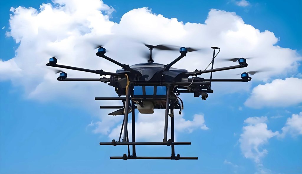
In this article, I address the UAV path planning problem with altitude windows by formulating it as a constrained optimization model and proposing a solution framework based on the Alternating Direction Method of Multipliers (ADMM). ADMM is a powerful algorithm that combines the benefits of dual decomposition and augmented Lagrangian methods, making it suitable for large-scale, non-convex problems like those involving UAV drones. By decomposing the original problem into smaller subproblems, ADMM enables efficient parallel computation and convergence to near-optimal solutions. This approach is particularly advantageous for UAV drones operating in dynamic environments where real-time adjustments may be needed.
The core contribution of this work lies in the development of a spatial network model that embeds altitude windows into the path planning process for UAV drones. This model minimizes total operational costs, including horizontal and vertical movement costs, while ensuring that each sampling region is serviced exactly once within its specified altitude range. To solve this model, I employ an ADMM-based framework that relaxes coupling constraints, decomposes the problem into independent subproblems for each UAV drone, and iteratively updates multipliers to achieve convergence. Numerical experiments using adapted benchmark datasets and real-world forestry data demonstrate the effectiveness of the proposed approach compared to traditional methods like Lagrangian relaxation.
This article is structured as follows: First, I describe the problem in detail and present the mathematical formulation. Then, I explain the theoretical foundations of ADMM and how it is applied to decompose the model. Next, I outline the solution algorithm, including a dynamic programming method with dominance rules. Subsequently, I present numerical results and sensitivity analyses. Finally, I conclude with key findings and future research directions. Throughout, I emphasize the relevance of UAV drones in modern applications and the importance of altitude-aware planning.
Problem Description and Modeling
The UAV path planning problem with altitude windows can be formally defined on a directed graph. Let \(G = (N, A)\) represent the physical network, where \(N\) is the set of nodes and \(A\) is the set of arcs. The nodes consist of sampling regions indexed as \(N_0 = \{1, 2, \dots, n\}\) and a depot node (split into start and end points, denoted as \(0\) and \(n+1\)). Each sampling region \(i \in N_0\) has an altitude window \([h_i^L, h_i^H]\), indicating the minimum and maximum allowable altitudes for UAV drones to collect samples. The arcs \((i, j) \in A\) represent possible paths between nodes, with associated costs: horizontal movement cost \(H_{i,j}\) and vertical movement cost \(V_{i,j}\). The vertical cost accounts for energy consumption during altitude changes, which is critical for UAV drones due to their limited battery life.
To incorporate altitude windows, I extend the physical network into a spatial network \(G_h = (N_h, A_h)\). Here, \(N_h\) includes nodes \((i, h)\) for each sampling region \(i\) and discrete altitude level \(h\) within the altitude set \(H = \{h_1, h_2, \dots, h_m\}\). The arcs \(((i, h), (j, h’)) \in A_h\) represent transitions from region \(i\) at altitude \(h\) to region \(j\) at altitude \(h’\), with costs combining horizontal and vertical components. This spatial representation allows UAV drones to dynamically adjust altitudes while traversing between regions, ensuring compliance with altitude windows.
The objective is to minimize the total cost for a fleet of UAV drones, denoted as set \(D\), where each UAV drone \(d \in D\) has a capacity \(q_d\) (e.g., weight or volume limit). Each sampling region \(i\) has a demand \(W_i\) (e.g., sample weight), and the UAV drones must satisfy all demands without exceeding their capacities. The decision variables are binary: \(x_{i,j,h,h’}^d = 1\) if UAV drone \(d\) travels from node \((i, h)\) to \((j, h’)\), and 0 otherwise. The mathematical model is formulated as follows:
Minimize the total cost:
$$ \min Z = \sum_{d \in D} \sum_{((i, h), (j, h’)) \in A_h} x_{i,j,h,h’}^d (H_{i,j,h,h’} + V_{i,j,h,h’}) $$
Subject to constraints:
Flow balance for each UAV drone \(d\):
$$ \sum_{((i, h), (j, h’)) \in A_h} x_{i,j,h,h’}^d – \sum_{((j, h’), (i, h)) \in A_h} x_{j,i,h’,h}^d = \begin{cases}
1 & \text{if } i = 0 \\
-1 & \text{if } i = n+1 \\
0 & \text{otherwise}
\end{cases} \quad \forall i \in N_h, d \in D $$
Each sampling region must be serviced exactly once by one UAV drone:
$$ \sum_{d \in D} \sum_{((i, h), (j, h’)) \in \psi_i} x_{i,j,h,h’}^d = 1 \quad \forall i \in N_0 $$
where \(\psi_i\) is the set of arcs incident to node \(i\).
Capacity constraints for UAV drones:
$$ w_j^d \geq w_i^d + W_j – M(1 – x_{i,j,h,h’}^d) \quad \forall i \in N_0, j \in N_0, d \in D $$
where \(w_i^d\) is the cumulative load of UAV drone \(d\) at node \(i\), and \(M\) is a large constant.
Binary decision variables:
$$ x_{i,j,h,h’}^d \in \{0, 1\} \quad \forall ((i, h), (j, h’)) \in A_h, d \in D $$
Altitude window constraints are implicitly enforced by the spatial network, as only altitudes within \([h_i^L, h_i^H]\) are included for node \(i\). This model captures the essential aspects of UAV drones operations in forestry surveys, but it is computationally challenging due to the combinatorial nature and coupling constraints.
Theoretical Foundations and Model Decomposition
To solve the UAV path planning model efficiently, I leverage the Alternating Direction Method of Multipliers (ADMM). ADMM is an iterative algorithm that blends dual decomposition and augmented Lagrangian methods, making it ideal for distributed optimization. The key idea is to decompose a complex problem into smaller, manageable subproblems that can be solved in parallel, which is beneficial for coordinating multiple UAV drones. In contrast to traditional Lagrangian relaxation, ADMM includes a quadratic penalty term in the objective function, which improves convergence and stability.
The standard ADMM addresses problems of the form:
$$ \min f(x) + g(z) \quad \text{s.t.} \quad Ax + Bz = c $$
where \(f\) and \(g\) are convex functions, and \(x\) and \(z\) are variable blocks. The augmented Lagrangian is:
$$ L_\rho(x, z, \lambda) = f(x) + g(z) + \lambda^T (Ax + Bz – c) + \frac{\rho}{2} \|Ax + Bz – c\|^2 $$
with penalty parameter \(\rho > 0\) and dual variable \(\lambda\). ADMM iterates by updating \(x\), \(z\), and \(\lambda\) alternately:
$$ x^{k+1} = \arg\min_x L_\rho(x, z^k, \lambda^k) $$
$$ z^{k+1} = \arg\min_z L_\rho(x^{k+1}, z, \lambda^k) $$
$$ \lambda^{k+1} = \lambda^k + \rho (Ax^{k+1} + Bz^{k+1} – c) $$
For the UAV drones problem, I extend ADMM to multiple blocks (one per UAV drone) due to the fleet size. This multi-block ADMM handles the coupling constraint that each sampling region must be serviced exactly once. By relaxing this constraint, the problem decomposes into independent subproblems for each UAV drone, linked through Lagrange multipliers.
Specifically, let the coupling constraint be \(\sum_{d \in D} \tau_i^d = 1\) for all \(i \in N_0\), where \(\tau_i^d\) is an indicator variable equal to 1 if UAV drone \(d\) services region \(i\), and 0 otherwise. The augmented Lagrangian relaxation of the original problem is:
$$ \min \sum_{d \in D} \left( \sum_{((i, h), (j, h’)) \in A_h} c_{i,j,h,h’}^d x_{i,j,h,h’}^d \right) + \sum_{i \in N_0} \lambda_i \left( \sum_{d \in D} \tau_i^d – 1 \right) + \frac{\rho}{2} \sum_{i \in N_0} \left( \sum_{d \in D} \tau_i^d – 1 \right)^2 $$
where \(c_{i,j,h,h’}^d = H_{i,j,h,h’} + V_{i,j,h,h’}\) is the cost for UAV drone \(d\). The quadratic term \(\frac{\rho}{2} \left( \sum_{d \in D} \tau_i^d – 1 \right)^2\) enhances convergence. To simplify, I linearize the quadratic term by introducing auxiliary variables and using the fact that \(\tau_i^d\) is binary. After linearization, the subproblem for each UAV drone \(d\) becomes a resource-constrained elementary shortest path problem (ESPPRC), which can be solved efficiently via dynamic programming.
The decomposition process involves iteratively solving each UAV drone’s subproblem while fixing other UAV drones’ variables, then updating the multipliers \(\lambda_i\). This approach parallels the coordination of multiple UAV drones in a fleet, where each UAV drone optimizes its own route based on shared global information. The ADMM framework ensures that solutions gradually satisfy the coupling constraints, yielding feasible paths for UAV drones.
Solution Algorithm
I propose a solution algorithm based on ADMM for UAV drones path planning. The algorithm consists of two main components: (1) solving the ESPPRC subproblems using dynamic programming with dominance rules, and (2) coordinating the subproblems via ADMM iterations to update multipliers and penalty parameters.
For each UAV drone \(d\), the subproblem is an ESPPRC on the spatial network \(G_h\), with modified arc costs that incorporate Lagrange multipliers and penalty terms. The cost for arc \(((i, h), (j, h’))\) in subproblem \(d\) is:
$$ \tilde{c}_{i,j,h,h’}^d = c_{i,j,h,h’}^d + \lambda_i + \rho \left( \tau_i^d – 0.5 \right) $$
where \(\tau_i^d\) is derived from the decision variables. This cost structure encourages UAV drones to cover regions that are under-served or over-served, balancing the workload across the fleet.
To solve the ESPPRC, I use a basic dynamic programming algorithm enhanced with dominance rules. Each partial path is represented by a label \((i, h, q, \Pi, C)\), where \(i\) is the current node, \(h\) is the current altitude, \(q\) is the cumulative load, \(\Pi\) is the set of visited nodes (to avoid cycles), and \(C\) is the accumulated cost. The algorithm expands labels from the depot to the end depot, respecting capacity and altitude constraints. Dominance rules prune inferior labels: a label \(L_1\) dominates \(L_2\) if \(C_1 \leq C_2\), \(q_1 \leq q_2\), and \(\Pi_1 \subseteq \Pi_2\). This reduces the state space and speeds up computation.
The overall ADMM-based algorithm for UAV drones is outlined in the following table, which summarizes the key steps and their purposes.
| Step | Description | Purpose |
|---|---|---|
| 1 | Initialize parameters: iteration count \(k=0\), multipliers \(\lambda^0\), penalty \(\rho^0\), upper bound \(UB^* = \infty\), lower bound \(LB^* = -\infty\). | Set up the iterative process for UAV drones coordination. |
| 2 | Solve Lagrangian relaxation subproblems for all UAV drones using dynamic programming to obtain a lower bound \(LB^k\). | Estimate the best possible cost for UAV drones routes. |
| 3 | Generate a feasible solution by adjusting subproblem solutions to satisfy coupling constraints; compute upper bound \(UB^k\). | Provide a practical route plan for UAV drones. |
| 4 | Update multipliers: \(\lambda_i^{k+1} = \lambda_i^k + \rho \left( \sum_{d \in D} \tau_i^d – 1 \right)\). | Penalize violations of the coupling constraint for UAV drones. |
| 5 | Adjust penalty parameter \(\rho\) based on convergence metrics (e.g., primal and dual residuals). | Improve convergence speed for UAV drones optimization. |
| 6 | Check stopping criteria: if gap \(Gap = \frac{UB^* – LB^*}{UB^*} \times 100\% \leq \epsilon\) or \(k \geq k_{\max}\), terminate; else, \(k = k+1\) and go to Step 2. | Ensure solution quality for UAV drones paths. |
This algorithm efficiently handles the path planning for multiple UAV drones by decomposing the problem and iteratively refining solutions. The dynamic programming component ensures optimality for each UAV drone’s subproblem, while ADMM coordinates the fleet to achieve a global near-optimum.
Numerical Experiments
To validate the proposed model and algorithm for UAV drones, I conduct numerical experiments using two datasets: (1) an adapted Solomon benchmark dataset, and (2) real-world data from a forested area in Nanjing, China. The experiments compare the ADMM-based framework with traditional Lagrangian relaxation in terms of solution quality, computational time, and convergence.
For the Solomon dataset, I modify instances by interpreting time windows as altitude windows for UAV drones. The instances include R101 and RC101 categories, with 25, 50, and 100 sampling regions. The fleet size is set to 25 UAV drones, each with a capacity of 100 units. Parameters: initial multipliers \(\lambda = 0\), penalty \(\rho = 1\), maximum iterations 100. The results are summarized in the table below, showing lower bound (LB), upper bound (UB), and computation time for both methods.
| Instance | Method | LB | UB | Time (s) | Gap (%) |
|---|---|---|---|---|---|
| r101.25 | Lagrangian | 511.4 | 651.4 | 7.77 | 21.5 |
| r101.25 | ADMM | 516.0 | 519.4 | 4.98 | 0.65 |
| r101.50 | Lagrangian | 523.0 | 1746.0 | 35.51 | 70.05 |
| r101.50 | ADMM | 864.0 | 908.0 | 20.49 | 4.85 |
| r101.100 | Lagrangian | 1052.1 | 2921.2 | 441.47 | 63.98 |
| r101.100 | ADMM | 1533.6 | 1540.1 | 379.97 | 0.42 |
| rc101.25 | Lagrangian | 622.9 | 778.8 | 5.97 | 19.90 |
| rc101.25 | ADMM | 570.0 | 575.3 | 3.97 | 0.92 |
| rc101.50 | Lagrangian | 1046.0 | 1632.0 | 36.30 | 35.91 |
| rc101.50 | ADMM | 1136.7 | 1150.3 | 32.92 | 1.18 |
| rc101.100 | Lagrangian | 1323.55 | 3044.13 | 564.31 | 56.52 |
| rc101.100 | ADMM | 1993.5 | 2053.5 | 454.03 | 2.92 |
The table clearly shows that the ADMM-based framework for UAV drones achieves significantly smaller gaps (average 1.82%) compared to Lagrangian relaxation (average 44.64%). This indicates that ADMM produces tighter bounds and more accurate solutions for UAV drones path planning. Moreover, ADMM is faster in most cases, especially for larger instances, highlighting its scalability for UAV drones fleets.
I also perform a sensitivity analysis on the penalty parameter \(\rho\) in ADMM for UAV drones. Using instance r101.25, I test values \(\rho \in \{0.2, 0.5, 1, 2, 4, 8\}\) and observe the convergence behavior. The results indicate that smaller \(\rho\) values lead to slower convergence but better solution quality, while larger \(\rho\) values speed up convergence at the cost of higher costs. Based on this, I recommend initializing \(\rho = 1\) for UAV drones problems, as it balances speed and accuracy.
For the real-world Nanjing forest data, I consider 30 sampling regions and 6 UAV drones with capacity 0.5 kg and volume 1 m³. Costs include fixed costs (150 per UAV drone), transportation (12 per km), and altitude changes (1 per m ascent, 0.5 per m descent). The ADMM-based framework obtains a solution with total cost 5059, using 5 UAV drones, travel distance 3852 m, and ascent 207 m. In comparison, a local search heuristic yields cost 5264, demonstrating the superiority of ADMM for UAV drones in practical scenarios.
Conclusion
In this article, I have addressed the UAV path planning problem with altitude windows, which is crucial for applications like forestry surveys using UAV drones. By formulating a spatial network model that incorporates altitude constraints, I capture the unique challenges of operating UAV drones in heterogeneous environments. The proposed ADMM-based solution framework effectively decomposes the problem into manageable subproblems for each UAV drone, enabling efficient coordination and convergence to near-optimal solutions.
The numerical experiments confirm that ADMM outperforms traditional Lagrangian relaxation in terms of solution quality and computational efficiency for UAV drones. The gaps between upper and lower bounds are significantly reduced, indicating robust performance. Sensitivity analysis highlights the importance of tuning the penalty parameter to balance convergence speed and accuracy for UAV drones.
Future work could extend this approach to more dynamic scenarios for UAV drones, such as real-time path adjustments due to weather changes or unexpected obstacles. Additionally, integrating energy consumption models and multiple objectives (e.g., minimizing time and risk) would enhance the practicality for UAV drones operations. The ADMM framework is flexible and can be adapted to these complexities, making it a valuable tool for advanced UAV drones path planning.
Overall, this research contributes to the optimization of UAV drones fleets in resource-constrained environments, paving the way for smarter and more sustainable autonomous systems. As UAV drones become increasingly prevalent, such algorithmic advancements will play a key role in unlocking their full potential across various industries.