
The evolution of integrated three-dimensional transportation networks and the accelerating deployment of low-altitude economy initiatives necessitate a paradigm shift in traffic governance—from roadside-centric passive perception to proactive, air-ground coordinated control. In this context, highways, especially on-ramp weaving sections, are prone to generating self-exciting and propagable stop-and-go waves. These waves significantly degrade traffic efficiency and increase energy consumption. Recent simulation studies have demonstrated the potential to suppress traffic flow oscillations by controlling a small fraction of vehicles, highlighting the promise of achieving collective stability with minimal intervention. To realize this potential in future transportation systems, a critical challenge must be addressed: seamlessly linking upstream global, accurate, and real-time observation with downstream rapid, smooth, and safe execution of control commands.
Unmanned Aerial Vehicles (UAV drones) offer a transformative solution for upstream observation. Their high mobility, wide field-of-view, and low deployment threshold provide an unobstructed, god’s-eye perspective of traffic dynamics. This capability is crucial for continuously tracking long-distance, cross-lane propagating phenomena like stop-and-go waves, which would otherwise require an expensive and dense network of roadside sensors. In the foreseeable transition period, the penetration rate of Connected and Automated Vehicles (CAVs) will likely remain low. Relying solely on sparse CAV data is insufficient for accurately reconstructing the continuous spatiotemporal evolution of traffic waves. UAV drones complement this by observing all vehicles within their visual range indiscriminately, generating complete and dense traffic flow information essential for effective group coordination under low CAV penetration rates. On the ground, CAVs, with their perception, communication, and controlled execution capabilities, serve as ideal actuators for implementing gentle speed-stabilization interventions. The open-source microscopic traffic simulation platform SUMO and its Traffic Control Interface (TraCI) provide a reliable and replicable testbed for rapidly iterating and evaluating such wave-absorption strategies. This paper, therefore, conducts research on stop-and-go wave mitigation for on-ramp weaving sections within an air-ground coordination scenario, proposing and validating a verifiable control strategy with performance assessment.
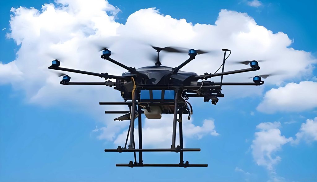
The high-altitude perspective provided by UAV drones is instrumental in overcoming the limitations of ground-based sensors. Their ability to cover large areas without obstruction makes them uniquely suited for capturing the ‘big picture’ of dynamic traffic phenomena, such as the formation and propagation of congestion waves at merge bottlenecks. This aerial vantage point is a key enabler for the coordinated framework proposed in this study.
1. Research Framework and Problem Formulation
This research establishes a replicable technical pathway from aerial observability to ground controllability for highway on-ramp weaving sections. Centered on the coordination of multiple UAV drones and a small number of CAVs, it forms an integrated framework for identification, prediction, control, and evaluation, with an ‘Arrival Time Window’ serving as the unifying interface.
1.1 Research Scenario and Observability
The scenario is a unidirectional highway on-ramp weaving section (mainline: two lanes). The objective is to establish a unified longitudinal road coordinate system and achieve continuous observation across multiple UAV drones’ fields of view (FoVs). Let time be \(t\) and the longitudinal road coordinate be \(s\), with downstream as the positive direction. There are \(M\) coordinating UAV drones (index \(i = 1, 2, …, M\)). The FoV of the \(i\)-th UAV drone at time \(t\) covers the longitudinal interval \([s_{i}^{-}(t), s_{i}^{+}(t)]\), where \(s_{i}^{-}(t)\) and \(s_{i}^{+}(t)\) are the upstream and downstream boundaries, respectively. The coverage length is \(L_i(t) = s_{i}^{+}(t) – s_{i}^{-}(t)\). Within this interval, \(N_i(t)\) vehicles are observed, with the instantaneous speed of the \(m\)-th vehicle being \(v_{i,m}(t)\) (unit: m/s). The sampling interval is \(\Delta t\).
To align multi-view data, let the road main axis unit vector be \(\mathbf{r}\) and the longitudinal zero point be \(\mathbf{x}_0\). The longitudinal coordinate \(s\) for any spatial point \(\mathbf{x}\) is defined as \(s = \mathbf{r}^\top (\mathbf{x} – \mathbf{x}_0)\). This unified coordinate supports all subsequent observation, estimation, and identification. To ensure continuity, let the wave propagation speed be \(c\), the minimum longitudinal overlap between adjacent FoVs be \(d_o\), and the maximum allowable time gap for cross-FoV arrival be \(T_{gap}\). To prevent the same wave event from being split, the condition \(d_o \geq c T_{gap}\) must be satisfied.
1.2 Macroscopic Variable Estimation
On the unified coordinate, macroscopic variables within each FoV are estimated using spatial averaging. The density \(k_i(t)\), space-mean speed \(u_i(t)\), and flow \(q_i(t)\) for the \(i\)-th FoV are defined as:
$$ k_i(t) = \frac{N_i(t)}{L_i(t)} $$
$$ u_i(t) = \left( \frac{1}{N_i(t)} \sum_{m=1}^{N_i(t)} \frac{1}{v_{i,m}(t)} \right)^{-1} $$
$$ q_i(t) = k_i(t) \cdot u_i(t) $$
The harmonic mean for speed provides a more accurate reflection of travel time efficiency under heterogeneous speeds, especially during congestion. A first-order exponential smoothing is applied to any scalar sequence \(x(t)\) (e.g., \(N_i(t)\), \(L_i(t)\)) to mitigate measurement noise: \(x_{\text{sm}}(t) = \rho x(t) + (1-\rho) x_{\text{sm}}(t-\Delta t)\), where \(\rho = \exp(-\Delta t / \tau)\) and \(\tau > 0\) is the time constant. Adaptive reference values for speed \(u_0(t)\) and density \(k_0(t)\) are defined using percentile operations over a historical window \(T_0\) to account for slow state drift.
1.3 Congestion Severity and Identification Delay
A congestion severity index \(S_i(t)\) is defined to measure significant speed drop and density increase:
$$ S_i(t) = \alpha \frac{u_0(t) – u_i(t)}{u_0(t)} + \beta \frac{k_i(t) – k_0(t)}{k_0(t)} $$
where \(\alpha, \beta \in (0,1)\) and \(\alpha + \beta = 1\). Its smoothed version is \(S_{i,\text{sm}}(t)\). Hysteresis thresholds are used for wave detection: a wave is triggered if \(S_{i,\text{sm}}(t) \geq S_{thr}\) for a duration \(T_{on}\), and it ends if \(S_{i,\text{sm}}(t) \leq S_{rel}\) for \(T_{off}\) or if valid samples are missing for \(T_{blk}\). A slow-vehicle proportion \(\phi_i(t)\) is also monitored, and triggering requires \(\phi_i(t) \geq \phi_{\min}\). The identification delay \(T_{det}\) can be approximated based on the smoothing dynamics and threshold settings.
1.4 Event-Based Representation and Control Target
A stop-and-go wave is described as an observable event sequence \(\epsilon_j\), represented by a triple \(\epsilon_j = (t_j, s_j, i_j)\), denoting its time, longitudinal position, and the index of the FoV where it was first observed. Its lifecycle is characterized by duration \(D = t_e – t_0\) and longitudinal span \(R = s_e – s_0\). The wave propagation speed \(c\) is theoretically given by the kinematic wave theory: \(c = (q_2 – q_1)/(k_2 – k_1)\). The integrated control objective is to minimize identification/response delay and the spatiotemporal scale of congestion by suppressing upstream propagating waves, thereby improving traffic efficiency, while satisfying all safety and feasibility constraints.
2. A Multi-UAV Drone Method for Full-Lifecycle Stop-and-Go Wave Identification
This section details the algorithm for identifying waves using data from a fleet of UAV drones.
2.1 Input and Output
Input: At each time \(t\), for each FoV \(i\): boundaries \([s_i^-, s_i^+]\), number of vehicle samples \(N_i\), set of vehicle speeds \(\{v_{i,m}\}\), and macroscopic variables \(k_i, u_i, q_i\).
Output: A set of identified waves \(W\). For each wave \(w \in W\), output its event sequence \(\epsilon(w) = \{(t_j, s_j, i_j)\}\), estimated wave speed \(\hat{c}\), statistics (direction, duration, span), and for any target location \(s^*\), the predicted arrival time window \([t_{\text{start}}, t_{\text{end}}]\).
2.2 Wave Front Extraction
The set of slow vehicles in FoV \(i\) is \(V_i(t) = \{m: v_{i,m}(t) \leq g \cdot u_f\}\), where \(u_f\) is the free-flow speed and \(g \in (0,1)\) is a threshold coefficient. The wave’s quantile front \(s_f(t)\) is defined as the \(\theta_f\)-percentile of the longitudinal positions of vehicles in \(V_i(t)\): \(s_f(t) = \text{perc}_{\theta_f}\{s_{i,m}(t): m \in V_i(t)\}\). Using \(\theta_f \approx 0.20\) and smoothing with time constant \(\tau_{sf} \sim 1s\) yields a robust representation of the wave front, \(s_{f,\text{sm}}(t)\). Quality checks are applied to reject events based on minimum sample size \(N_{\min}\) and minimum slow-vehicle proportion \(\phi_{\min}\).
2.3 Cross-FoV Association and Wave Speed Estimation
A cooling time \(T_{cool}\) prevents duplicate triggering. For a new candidate event \((t, s)\), the algorithm first attempts to attach it to an existing wave. Let the latest event of an existing wave be \((t_l, s_l)\). A predicted position is calculated using a historically estimated wave speed \(c_h\): \(s_{\text{pred}} = s_l + c_h (t – t_l)\). If the residual \(|s – s_{\text{pred}}| \leq r_{\text{attach}}\), attachment occurs. A recently ended wave can also be resurrected within a spatiotemporal window. Wave speed is estimated by fusing three methods: 1) Full-history linear regression slope \(c_h\), 2) Sliding-window regression slope \(c_w\), and 3) LWR-based speed \(c_l\) derived from a recent two-phase clustering of vehicle speeds. The final robust estimate \(\hat{c}\) is the median of these available estimates, and the propagation direction is determined by its sign.
2.4 Wave Termination, Summarization, and Arrival Time Window
A wave is terminated if no new event attaches to it for a duration corresponding to \(T_{off}\). Its statistics are then summarized. For the latest event \((t_l, s_l)\) of an active wave and a target upstream location \(s^*\), the arrival time window is calculated using the lower and upper percentiles (e.g., 25th and 75th) of the collected wave speed estimates, \(\hat{c}_-\) and \(\hat{c}_+\):
$$ t_{\text{start}} = t_l + \frac{s^* – s_l}{\hat{c}_+}, \quad t_{\text{end}} = t_l + \frac{s^* – s_l}{\hat{c}_-}, \quad \Delta t^* = t_{\text{end}} – t_{\text{start}} $$
This window \([t_{\text{start}}, t_{\text{end}}]\) is the key output bridging identification and control, providing the time interval during which a wave is expected to pass the control point.
3. UAV-Assisted Jam-Absorption Driving Control Method
This section describes how the identified wave information is used to control CAVs to absorb the congestion.
3.1 Control Objective and Constraints
The control objective is to prevent the inflow demand from exceeding the downstream bottleneck capacity, causing the wave’s amplitude and spatial extent to decay. CAV dynamics and management constraints include maximum acceleration \(a_{\max}\), maximum deceleration \(a_{\min}\) (negative), minimum headway \(h_{\min}\), speed limit \(u_{\max}\), and a control time budget accounting for communication and execution delays.
3.2 Trigger and Control Position (Event-Driven)
Upon receiving an arrival time window \([t_{\text{start}}, t_{\text{end}}]\) at target location \(s^*\) from the identification layer, the controller selects a trigger time \(t^\dagger\) within this window. The required distance \(\Delta\) upstream of \(s^*\) to place a controlled CAV is calculated as \(\Delta = (u^* – \hat{c}) T_h\), where \(u^*\) is the target speed for the absorbing CAV and \(T_h\) is the control horizon. The distance \(\Delta\) is clipped to a feasible range \([50\text{m}, 0.6 L_{\text{FoV}}]\). The controller then selects a suitable CAV within the spatiotemporal window defined by \(t^\dagger\) and \(\Delta\) to execute the control.
3.3 Jam-Absorption Control Strategy
For the selected CAV at position \(s_a(t)\), traffic parameters are estimated in an upstream window \([s_a – L_\uparrow, s_a]\) and a forward window \([s_a, s_a + L_\downarrow]\), denoted as \((k_\uparrow, u_\uparrow, q_\uparrow)\) and \((k_\downarrow, u_\downarrow, q_\downarrow)\) respectively. The target speed \(u^*\) for the absorbing CAV is set to match the downstream flow-to-density ratio, stabilized to avoid flow breakdown: \(u^* = \max(q_\uparrow / (k_\downarrow + \sigma), u_\downarrow)\), where \(\sigma > 0\) is a small constant. This value is clipped to \([0, u_{\text{free}}]\). Speed commands are smoothed using a first-order convex combination with rate limiting:
$$ u_{\text{cmd}}(t) = \gamma u^* + (1-\gamma) u_{\text{base}}(t) $$
$$ u_{\text{cmd}}(t) \in [u_{\text{prev}}(t-\Delta t) + a_{\min} \Delta t, \quad u_{\text{prev}}(t-\Delta t) + a_{\max} \Delta t] $$
where \(\gamma \in (0,1)\) is a smoothing weight, and \(u_{\text{base}}(t)\) is an inertial baseline speed. When the distance to the wave front exceeds a release threshold \(d_{\text{rel}}\) or the forward window is cleared (based on vehicle count and speed/density hysteresis), the CAV switches to a recovery mode with a higher acceleration limit to smoothly return to the desired speed.
3.4 Stability and Feasibility
Under a triangular fundamental diagram \(Q(k)\), if the control ensures the controlled inflow \(q_{\uparrow, \text{ctrl}} = k_\uparrow u^* \leq Q(k_\downarrow)\), then the accumulation in the congested region does not increase, leading to monotonic decay of the wave. Feasibility depends on identification accuracy, vehicle dynamic limits, and geometric reachability, all of which are incorporated into the control design via the time window, rate limits, and horizon \(T_h\).
4. Case Study and Analysis
The proposed framework is validated using the SUMO microscopic traffic simulator. The scenario is a highway on-ramp weaving section with a 230-meter acceleration lane. The demand consists of a mix of passenger cars and trucks with varying dynamics on both the mainline and the on-ramp, totaling 2960 veh/h, designed to create recurrent congestion at the merge point.
4.1 Experimental Setup and Benchmark Scenarios
Four scenarios are compared:
B0 (UAV Observation Only): Serves as the baseline with natural wave evolution.
B1 (Traditional V2I Absorption, 5% CAV): Uses fixed control rules based on wave speed, without time windows or multi-UAV event fusion.
B2 (Adaptive Dynamic Control, 2% CAV): Uses CAV-local sensing and adaptive rules, without the proposed UAV coordination framework.
B3 (Proposed UAV-CAV Coordination, 2% CAV): Implements the full framework: UAV drone identification, arrival time window prediction, and event-triggered absorption control.
Key algorithm hyperparameters are summarized in the table below.
| Parameter | Value | Description/Rationale |
|---|---|---|
| \(\Delta t\) | 0.2 s | Simulation step. Balances detail and computational efficiency. |
| \(M\) (UAV drones) | 2 | Provides full coverage of the key weaving section. |
| \(S_{thr}, S_{rel}\) | 0.60, 0.52 | Hysteresis thresholds for robust congestion state detection. |
| \(T_{on}, T_{off}\) | 4 s | Minimum duration for state confirmation; filters transient noise. |
| \(\phi_{\min}\) | 0.4 | Minimum slow-vehicle proportion. Ensures congestion is a collective phenomenon. |
| \(g\) | 0.6 | Slow-vehicle threshold coefficient. Vehicles below 60% of free-flow speed are considered “slow”. |
| \(T_{cool}\) | 10 s | Cooling time per FoV to prevent duplicate wave creation. |
4.2 Wave Identification Results
The identification algorithm successfully detected multiple stop-and-go waves over a 1000-second simulation. The detected waves showed upstream propagation (negative wave speeds), with durations varying from 16 to 183 seconds. The median speed within the waves ranged from 1 to 3 m/s, and the median congestion severity \(S\) ranged from 0.56 to 0.67, confirming the capture of significant low-speed, high-density events. The start times of identified waves visually matched the appearance of red (low-speed) bands in the spacetime trajectory diagram, validating the identification accuracy.
4.3 Control Performance Analysis
The efficiency gains of the control strategies are summarized in the table below. The proposed UAV-CAV coordinated strategy (B3) achieves the best overall performance, even with only a 2% CAV penetration rate.
| Scenario | Avg. Travel Time (s) & Change | Avg. Waiting Time (s) & Change | Avg. Fuel (L/100km) & Change |
|---|---|---|---|
| B0 (Baseline) | 65.78 | 0.684 | 11.78 |
| B1 (V2I, 5%) | 64.80 (-1.5%) | 0.677 (-1.0%) | 11.60 (-1.5%) |
| B2 (Adaptive, 2%) | 64.53 (-1.9%) | 0.673 (-1.6%) | 11.53 (-2.1%) |
| B3 (Proposed, 2%) | 63.71 (-3.1%) | 0.670 (-2.0%) | 11.37 (-3.5%) |
Wave-level analysis confirms these trends. As shown in Figure 1, the proposed strategy B3 consistently reduces the congestion severity \(S\) and increases the median speed within waves compared to the baseline B0 and the other benchmarks B1 and B2. This indicates that the control effectively dampens the amplitude of speed oscillations and mitigates the severity of the stop-and-go waves.
A vehicle-type analysis reveals heterogeneous effects. The strategy significantly benefits standard passenger cars and trucks, reducing their travel time and waiting time. However, for inherently slow vehicles (e.g., slow trucks), the stabilizing control can slightly increase their travel delay, suggesting the need for differentiated or less aggressive control parameters for such vehicle classes in practical implementation.
4.4 Sensitivity to UAV Drone Deployment
The robustness of the framework was tested against different UAV drone deployment strategies. Three scenarios were compared: 1) Baseline (2 UAV drones, full coverage), 2) High Redundancy (3 UAV drones), and 3) Coverage Gap (2 UAV drones with a blind zone). The results, summarized below, show that full coverage is critical. The high-redundancy scenario offered negligible extra benefit over the baseline, indicating the 2-UAV setup is cost-effective. The coverage gap scenario led to significant performance degradation (travel time increase of ~2.0%), as wave tracking and prediction accuracy suffered when the wave passed through the unobserved region.
| Deployment Scenario | Avg. Travel Time (s) | Performance Note |
|---|---|---|
| 1. Baseline (2 UAV, Full Cover) | 63.71 | Reference performance. |
| 2. High Redundancy (3 UAV) | 63.59 | Marginal gain (<0.5%), diminishing returns. |
| 3. Coverage Gap (2 UAV, Blind Zone) | 64.97 | Significant loss (~2.0%). Highlights need for continuous observation. |
5. Conclusion
This paper presented a novel, integrated air-ground coordination framework for mitigating stop-and-go waves in highway on-ramp weaving sections. The framework leverages the high-altitude, wide-area observational capabilities of multiple UAV drones to achieve full-lifecycle identification and prediction of congestion waves, and uses a small fraction of CAVs as ground actuators to execute a gentle, event-triggered jam-absorption driving strategy. The key innovation is the use of a unified ‘Arrival Time Window’ as the interface between perception and control, reducing latency and strategy drift.
Simulation results demonstrate that the proposed UAV-CAV coordinated strategy can reduce average travel time by approximately 3.1% and fuel consumption by 3.5% compared to a no-control baseline, even under a low CAV penetration rate of 2%. Wave-level metrics confirm a reduction in congestion severity and a stabilization of speeds. The study highlights that the synergy between UAV drone-provided global observability and CAV-executed localized control offers a practical and cost-effective solution for traffic wave management in the transitional period towards full automation, without relying on heavy roadside infrastructure. The framework is compatible with existing strategies like Variable Speed Limits and ramp metering.
Limitations and Future Work: The study assumes idealized perception and communication; incorporating explicit models for UAV drone observation noise and communication delays is a necessary next step. The control parameters showed heterogeneous effects across vehicle types, indicating a need for differentiated control strategies. Future research will focus on: 1) Transitioning from simulation to field tests for real-world validation; 2) Joint optimization of identification and control parameters under uncertainty; and 3) Developing multi-UAV drone fleet scheduling algorithms to optimize coverage, latency, and energy consumption for large-scale network applications.