
In recent years, the quadrotor drone has evolved from a specialized research platform to a ubiquitous tool with applications spanning from aerial photography and agricultural monitoring to search and rescue and infrastructure inspection. At the heart of any quadrotor drone‘s capability lies its flight control system—a sophisticated set of algorithms that interpret pilot commands or autonomous mission objectives and translate them into precise motor actuation. This system is responsible for maintaining stability, enabling agile maneuvers, and rejecting disturbances. However, designing effective controllers for a quadrotor drone is inherently challenging due to its complex dynamics. This article provides a detailed, first-person perspective exploration of the mathematical modeling, control architectures, and the diverse array of flight control algorithms developed for quadrotor drones.
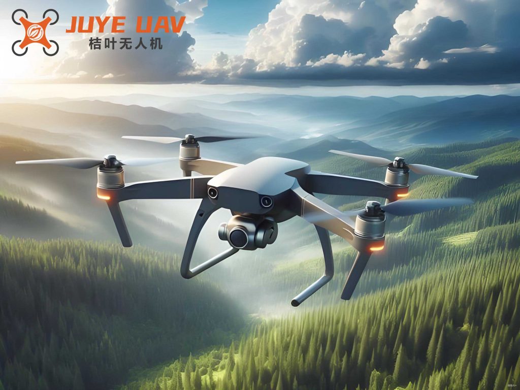
The fundamental challenge in controlling a quadrotor drone stems from its nature as an underactuated, highly nonlinear, and strongly coupled system. It possesses six degrees of freedom (position and orientation in three-dimensional space) but only four independent control inputs (the thrusts of its four rotors). Furthermore, achieving precise control is complicated by parametric uncertainties (e.g., mass, inertia), unmodeled dynamics (e.g., aerodynamic drag, motor dynamics), and external disturbances (e.g., wind gusts). Researchers have approached this problem from various angles, leading to a rich taxonomy of control strategies, each with its own merits and trade-offs concerning performance, robustness, and implementation complexity.
1. Mathematical Modeling of the Quadrotor Drone
Any control design must begin with a mathematical model. We define two coordinate frames: the body-fixed frame \( B \) attached to the quadrotor drone‘s center of mass, and the inertial earth frame \( E \). The orientation of the quadrotor drone is described by the Z-Y-X Euler angles \( \boldsymbol{\eta} = [\phi, \theta, \psi]^T \), representing roll, pitch, and yaw, respectively. The position of the center of mass in the inertial frame is given by \( \boldsymbol{\xi} = [x, y, z]^T \).
The equations of motion can be derived using the Newton-Euler or Euler-Lagrange formalisms. The translational dynamics in the inertial frame are:
$$
m \ddot{\boldsymbol{\xi}} = \boldsymbol{R} \begin{bmatrix} 0 \\ 0 \\ F_{total} \end{bmatrix} – \begin{bmatrix} 0 \\ 0 \\ mg \end{bmatrix} + \boldsymbol{d}_{trans}
$$
where \( m \) is the mass, \( g \) is gravitational acceleration, \( F_{total} = \sum_{i=1}^{4} F_i \) is the total thrust from all four rotors, \( \boldsymbol{R} \in SO(3) \) is the rotation matrix from frame \( B \) to \( E \), and \( \boldsymbol{d}_{trans} \) represents external disturbance forces.
The rotational dynamics are more conveniently expressed in the body frame to maintain a constant inertia matrix:
$$
\boldsymbol{I} \dot{\boldsymbol{\omega}}^B = – \boldsymbol{\omega}^B \times (\boldsymbol{I} \boldsymbol{\omega}^B) + \boldsymbol{\tau} + \boldsymbol{d}_{rot}
$$
where \( \boldsymbol{\omega}^B = [p, q, r]^T \) is the angular velocity vector in the body frame, \( \boldsymbol{I} = \text{diag}(I_{xx}, I_{yy}, I_{zz}) \) is the inertia matrix, \( \boldsymbol{\tau} = [\tau_\phi, \tau_\theta, \tau_\psi]^T \) are the control torques about the body axes, and \( \boldsymbol{d}_{rot} \) represents disturbance torques. The relationship between the Euler angle rates and the body angular rates is given by:
$$
\dot{\boldsymbol{\eta}} = \boldsymbol{J}(\boldsymbol{\eta}) \boldsymbol{\omega}^B, \quad \boldsymbol{J}(\boldsymbol{\eta}) = \begin{bmatrix}
1 & \sin\phi \tan\theta & \cos\phi \tan\theta \\
0 & \cos\phi & -\sin\phi \\
0 & \sin\phi \sec\theta & \cos\phi \sec\theta
\end{bmatrix}
$$
The control inputs \( (F_{total}, \boldsymbol{\tau}) \) are generated by varying the speeds of the four rotors \( \Omega_i \). Assuming a simple model where thrust \( F_i = k_F \Omega_i^2 \) and drag torque \( Q_i = k_Q \Omega_i^2 \) are proportional to the square of rotor speed, the mapping from rotor speeds to body forces and torques is:
$$
\begin{bmatrix}
F_{total} \\ \tau_\phi \\ \tau_\theta \\ \tau_\psi
\end{bmatrix}
=
\begin{bmatrix}
k_F & k_F & k_F & k_F \\
0 & -L k_F & 0 & L k_F \\
-L k_F & 0 & L k_F & 0 \\
k_Q & -k_Q & k_Q & -k_Q
\end{bmatrix}
\begin{bmatrix}
\Omega_1^2 \\ \Omega_2^2 \\ \Omega_3^2 \\ \Omega_4^2
\end{bmatrix}
$$
where \( L \) is the distance from the center of mass to a rotor. This model reveals the inherent coupling and underactuation: the four rotor speeds control four generalized forces (one total thrust and three torques), leaving two translational degrees of freedom (horizontal motion) indirectly controlled via attitude tilting.
| Model Parameter | Symbol | Typical Role in Dynamics |
|---|---|---|
| Mass | \( m \) | Directly scales translational inertia and required thrust. |
| Inertia Matrix | \( \boldsymbol{I} \) | Determines rotational acceleration for a given torque. |
| Thrust Coefficient | \( k_F \) | Maps rotor speed squared to thrust force. |
| Drag Coefficient | \( k_Q \) | Maps rotor speed squared to reactive drag torque. |
| Arm Length | \( L \) | Lever arm determining torque generation efficiency. |
| Aerodynamic Drag Coeff. | \( k_D \) | Models velocity-dependent drag force, often added as \( -k_D \dot{\boldsymbol{\xi}} \). |
2. Control Architecture for Quadrotor Drones
Given the underactuated nature of the quadrotor drone, a hierarchical, cascaded control structure is almost universally employed. This structure decomposes the problem into an outer-loop (position/velocity) controller and an inner-loop (attitude) controller.
- Outer-Loop (Position Control): This controller takes the desired trajectory \( \boldsymbol{\xi}_d(t), \dot{\boldsymbol{\xi}}_d(t) \) as input and generates a desired attitude \( (\phi_d, \theta_d) \) and a desired total thrust \( F_{total, d} \). From the translational dynamics, we see that horizontal acceleration is achieved by tilting the thrust vector. By solving for the required tilt angles, the position controller outputs virtual commands.
- Inner-Loop (Attitude Control): This is the high-bandwidth, high-precision core of the flight controller. It takes the desired attitude \( (\phi_d, \theta_d, \psi_d) \) and desired thrust \( F_{total, d} \) from the outer loop and computes the required control torques \( \boldsymbol{\tau} \). These torques, along with the thrust, are then mapped to individual motor commands via the control allocation matrix.
The yaw angle \( \psi \) is often controlled independently within the attitude loop, as it does not directly affect horizontal translation in a linearized sense. This cascaded approach simplifies design by allowing separate controller tuning for the slower translational dynamics and the faster rotational dynamics. Robustness of the inner loop is paramount, as any attitude tracking error directly corrupts the translational control effort.
3. Flight Control Algorithms for Quadrotor Drones
The following sections delve into the principal categories of control algorithms developed for quadrotor drones.
3.1. Classical PID Control
The Proportional-Integral-Derivative (PID) controller remains the workhorse in commercial and many research quadrotor drone platforms due to its simplicity, intuitive tuning, and proven effectiveness for linear or mildly nonlinear systems. The control law for a generic error \( e(t) \) is:
$$
u(t) = K_p e(t) + K_i \int_0^t e(\tau) d\tau + K_d \frac{de(t)}{dt}
$$
For a quadrotor drone, separate PID controllers are designed for each axis in both the inner and outer loops. For the attitude loop (inner loop), considering the roll channel as an example under small-angle assumptions:
$$
\tau_\phi = K_{p,\phi} (\phi_d – \phi) + K_{i,\phi} \int (\phi_d – \phi) dt + K_{d,\phi} (\dot{\phi}_d – \dot{\phi})
$$
The position loop (outer loop) generates desired angles. For the \( x \)-channel:
$$
\theta_d = K_{p,x} (x_d – x) + K_{i,x} \int (x_d – x) dt + K_{d,x} (\dot{x}_d – \dot{x})
$$
The total thrust command is typically generated from the altitude \( z \)-channel PID output. While simple, a major drawback is the need to manually tune up to 18 parameters (3 gains × 3 attitude axes × 2 loops). Performance degrades significantly under aggressive maneuvers (where nonlinearities dominate) or in the presence of persistent disturbances, as the fixed-gain linear feedback lacks adaptation mechanisms.
| Aspect | Advantages | Disadvantages |
|---|---|---|
| Implementation | Extremely simple, low computational cost. | Parameter tuning is time-consuming and often ad-hoc. |
| Performance | Excellent for stabilization and gentle flight. | Poor robustness to model uncertainty and large disturbances. |
| Nonlinearity | Effective for linearized models around hover. | Performance degrades during aggressive, nonlinear flight regimes. |
| Industry Use | Dominant algorithm in consumer and many commercial drones. | Often augmented with feedforward or adaptive terms for better performance. |
3.2. Linear Quadratic Regulator (LQR) Control
The Linear Quadratic Regulator (LQR) is an optimal state-feedback control technique for linear systems. It provides a systematic method for designing a controller that minimizes a quadratic cost function, balancing state error and control effort. For the linearized state-space model of a quadrotor drone:
$$
\dot{\boldsymbol{x}} = \boldsymbol{A} \boldsymbol{x} + \boldsymbol{B} \boldsymbol{u}
$$
where \( \boldsymbol{x} \) is the state vector (e.g., \( [x, \dot{x}, y, \dot{y}, z, \dot{z}, \phi, \dot{\phi}, \theta, \dot{\theta}, \psi, \dot{\psi}]^T \)) and \( \boldsymbol{u} \) is the control input vector (e.g., \( [F_{total}, \tau_\phi, \tau_\theta, \tau_\psi]^T \)), the LQR control law is:
$$
\boldsymbol{u} = -\boldsymbol{K} \boldsymbol{x}
$$
The gain matrix \( \boldsymbol{K} \) is obtained by solving the Algebraic Riccati Equation (ARE):
$$
\boldsymbol{A}^T \boldsymbol{P} + \boldsymbol{P} \boldsymbol{A} – \boldsymbol{P} \boldsymbol{B} \boldsymbol{R}^{-1} \boldsymbol{B}^T \boldsymbol{P} + \boldsymbol{Q} = \boldsymbol{0}
$$
where \( \boldsymbol{K} = \boldsymbol{R}^{-1} \boldsymbol{B}^T \boldsymbol{P} \). The matrices \( \boldsymbol{Q} \ge 0 \) and \( \boldsymbol{R} > 0 \) are design weights penalizing state deviations and control effort, respectively. The main advantage is the automatic computation of an optimal gain matrix once \( \boldsymbol{Q} \) and \( \boldsymbol{R} \) are chosen. However, LQR’s performance is tied to the accuracy of the linearized model \( (\boldsymbol{A}, \boldsymbol{B}) \). Significant nonlinearities or parameter variations can lead to suboptimal performance or even instability, limiting its use to near-hover conditions unless combined with gain scheduling or other nonlinear techniques.
3.3. Sliding Mode Control (SMC)
Sliding Mode Control is a robust nonlinear control technique particularly effective for systems with modeling uncertainties and bounded disturbances. The core idea is to force the system’s state trajectory onto a user-defined sliding surface \( s(\boldsymbol{x}) = 0 \) in the state space and then maintain it there using discontinuous control. Once on the surface, the system’s dynamics are governed by the surface equation, which is independent of system parameters and disturbances.
Design involves two steps: 1) Define a stable sliding surface. For a second-order attitude error \( e_\phi = \phi_d – \phi \), a common choice is:
$$
s_\phi = \dot{e}_\phi + \lambda_\phi e_\phi, \quad \lambda_\phi > 0
$$
2) Design a control law that ensures the reachability condition \( s \dot{s} < 0 \) is met. A typical SMC law for the quadrotor drone attitude loop has two parts:
$$
\tau_\phi = \tau_{\phi,eq} + \tau_{\phi,sw}
$$
The equivalent control \( \tau_{\phi,eq} \) is derived by setting \( \dot{s}_\phi = 0 \) assuming no disturbances. The switching control \( \tau_{\phi,sw} \) compensates for uncertainties and disturbances, often taking the form:
$$
\tau_{\phi,sw} = -K_{\phi} \cdot \text{sgn}(s_\phi)
$$
where \( \text{sgn}(\cdot) \) is the signum function. The major advantage is invariance to matched disturbances once in sliding mode. The primary drawback is chattering—high-frequency oscillations caused by the discontinuous signum function, which can excite unmodeled dynamics and wear actuators. This is often mitigated by using a continuous approximation like a saturation function \( \text{sat}(s/\Phi) \). Higher-order sliding mode controllers, like the super-twisting algorithm, can also attenuate chattering while preserving robustness.
3.4. Backstepping Control
Backstepping is a recursive Lyapunov-based design procedure for nonlinear systems in strict-feedback form. It is well-suited for the cascaded structure of the quadrotor drone dynamics. The method systematically constructs a control law and a Lyapunov function to guarantee global asymptotic stability.
Consider a simplified pitch dynamics model: \( \ddot{\theta} = f(\theta, \dot{\theta}) + g \cdot \tau_\theta \). The design proceeds stepwise:
- Step 1: Treat \( \dot{\theta} \) as a virtual control input \( \alpha_1 \) for the \( \theta \)-subsystem. Define error \( z_1 = \theta_d – \theta \). Choose a Lyapunov function \( V_1 = \frac{1}{2} z_1^2 \). Design \( \alpha_1 \) to stabilize this subsystem: \( \alpha_1 = c_1 z_1 + \dot{\theta}_d \), with \( c_1 > 0 \).
- Step 2: Define the error between the virtual control and its desired value: \( z_2 = \alpha_1 – \dot{\theta} \). Now consider the augmented Lyapunov function \( V_2 = V_1 + \frac{1}{2} z_2^2 \). Its derivative is:
$$ \dot{V}_2 = z_1(\dot{z}_1) + z_2(\dot{z}_2) = z_1(\dot{\theta}_d – \dot{\theta}) + z_2(\dot{\alpha}_1 – \ddot{\theta}) $$
Substitute the dynamics \( \ddot{\theta} = f + g\tau_\theta \):
$$ \dot{V}_2 = z_1(z_2 – c_1 z_1) + z_2(\dot{\alpha}_1 – f – g\tau_\theta) $$ - Step 3: Design the actual control input \( \tau_\theta \) to make \( \dot{V}_2 \) negative definite:
$$ \tau_\theta = \frac{1}{g} [ \dot{\alpha}_1 – f + z_1 + c_2 z_2 ], \quad c_2 > 0 $$
This yields \( \dot{V}_2 = -c_1 z_1^2 – c_2 z_2^2 < 0 \), proving asymptotic stability.
Backstepping provides a structured way to handle nonlinearities without cancellation, but it requires knowledge of the nonlinear functions \( f \) (i.e., an accurate model). This limitation has led to the development of adaptive backstepping and robust backstepping variants for quadrotor drone control.
3.5. Robust Control via Disturbance Observer (DOB)
Robust control strategies aim to maintain performance despite model uncertainties. A highly effective and practical approach for the quadrotor drone is to augment a nominal controller (like PID) with a Disturbance Observer (DOB). The DOB estimates the aggregate effect of model mismatch, nonlinearities, and external disturbances, and then injects a compensating control signal.
The core concept is to treat the actual plant \( P(s) \) as a nominal model \( P_n(s) \) plus an additive lumped disturbance \( d \): \( y = P(u + d) \). The DOB estimates \( d \) by comparing the actual output \( y \) with the output of the nominal model driven by the control input \( u \):
$$
\hat{d} = Q(s) [ P_n^{-1}(s) y – u ]
$$
where \( Q(s) \) is a low-pass filter (the Q-filter) with a bandwidth \( \omega_q \). It is crucial for realizability (making \( P_n^{-1}(s) \) proper) and noise attenuation. The estimated disturbance is then fed back to cancel itself:
$$
u = u_{nom} – \hat{d}
$$
Here, \( u_{nom} \) is the output of the nominal PID controller. The closed-loop system behaves like the nominal system for disturbances with frequency content below \( \omega_q \). This method significantly enhances the robustness of a standard quadrotor drone flight controller without requiring intricate redesign of the primary control law. The key design choice is the bandwidth of the Q-filter, which trades off disturbance rejection against robustness to measurement noise.
3.6. Other Advanced Control Methods
Beyond the core methods, other advanced algorithms have been applied to quadrotor drone control:
- Adaptive Control: These algorithms online estimate unknown or slowly varying parameters (e.g., mass, inertia, aerodynamic coefficients) and adjust the controller accordingly. Model Reference Adaptive Control (MRAC) and adaptive backstepping are common frameworks. They are powerful for handling payload changes but can have slow convergence and complex stability analyses.
- Model Predictive Control (MPC): MPC solves a finite-horizon optimal control problem online at each time step, explicitly handling state and input constraints. It is highly effective for trajectory tracking and obstacle avoidance but is computationally demanding for fast dynamics like those of a quadrotor drone, requiring powerful onboard processors.
- Learning-Based Control (Neural Networks, Fuzzy Logic): Neural Networks (NNs) can be used as universal approximators to learn inverse dynamics or compensate for unmodeled effects. Fuzzy Logic Controllers (FLC) use heuristic rule bases to map sensor inputs to control actions. Both can model complex nonlinearities without explicit equations but require extensive data/tuning and can lack formal stability guarantees, though this is an active research area.
| Algorithm Category | Key Strengths | Key Weaknesses | Suitability for Quadrotor Drones |
|---|---|---|---|
| PID | Simple, intuitive, computationally cheap. | Non-robust, poor for nonlinear flight. | Excellent for basic stabilization and commercial products. |
| LQR | Optimal for linear model, systematic design. | Performance limited to linear regime. | Good for near-hover control, often used in inner loops. |
| Sliding Mode | Very robust to matched disturbances. | Chattering, high control activity. | Excellent for robust attitude control, requires careful implementation. |
| Backstepping | Systematic nonlinear design, stability proof. | Requires accurate model, can be complex. | Well-suited for theoretical development and full nonlinear control. |
| Robust (e.g., DOB) | Enhances simple controllers, practical. | Adds design complexity (filter tuning). | Highly practical for improving real-world PID performance. |
| Adaptive / Learning | Handles uncertainties, can learn models. | Complexity, stability proofs, data needs. | Promising for advanced applications with varying conditions. |
4. Future Trends and Research Directions
The evolution of flight control for the quadrotor drone is moving beyond basic stabilization and trajectory tracking. Future trends are heavily influenced by demands for greater autonomy, intelligence, and coordination:
- Fault-Tolerant Control (FTC): Algorithms capable of detecting and accommodating actuator faults (e.g., motor failure, propeller damage) or sensor faults to ensure safe operation. This is critical for urban air mobility and safety-critical missions.
- Vision-Based and Sensor Fusion Control: Tight integration of vision (e.g., Visual SLAM, optical flow), LiDAR, and inertial sensors for navigation in GPS-denied environments. Control algorithms must handle the noise, latency, and intermittent nature of these sensing modalities.
- Agile and Acrobatic Flight: Control designs that exploit, rather than avoid, nonlinear dynamics to perform high-speed maneuvers, flips, and perching. This often involves hybrid control and trajectory optimization at the limits of actuator performance.
- Swarm Intelligence and Cooperative Control: Controlling large-scale fleets of quadrotor drones for collaborative tasks like mapping, formation flying, or search. This introduces challenges in distributed control, communication, and collective decision-making.
- Learning-Based Optimal Control: Merging MPC with machine learning (e.g., using NNs to approximate the optimal policy or value function) to reduce computational load while maintaining near-optimal performance for complex tasks.
5. Conclusion
The field of flight control for quadrotor drones represents a rich intersection of classical control theory and modern nonlinear and robust techniques. From the foundational simplicity of PID to the robust guarantees of sliding mode control and the structured nonlinearity handling of backstepping, each algorithm family offers distinct trade-offs. The choice of controller depends heavily on the application’s specific requirements: computational resources, required performance envelope, expected disturbances, and the need for formal guarantees. The cascaded inner-outer loop architecture remains a foundational paradigm. As the missions for quadrotor drones become more ambitious—demanding autonomy, resilience, and cooperation—the control algorithms will continue to evolve, increasingly blending model-based design with data-driven learning to create the next generation of intelligent aerial robots.