
The rapid development of e-commerce and the growing demand for instant logistics have propelled the exploration of innovative delivery methods. Unmanned Aerial Vehicle (UAV) delivery, characterized by its independence from ground traffic congestion, high speed, and relatively low operational costs, has emerged as a pivotal direction in the evolution of smart logistics systems. Efficiently planning delivery routes, which involves the scientific assignment of tasks, allocation of UAV resources, and optimization of flight paths, constitutes the core challenge in leveraging UAV technology for logistics. This task is inherently a complex resource scheduling and path optimization problem, often requiring the simultaneous consideration of multiple, often conflicting, objectives such as minimizing cost, maximizing timeliness, and ensuring service quality. Traditional approaches that aggregate multiple objectives into a single one using weighted sums rely heavily on empirical weight settings and fail to reveal the inherent trade-offs between objectives. To address this gap, this paper formulates the UAV delivery task allocation problem as a genuine multi-objective optimization model. The model simultaneously minimizes total weighted flight distance, minimizes robust completion time, and maximizes the demand satisfaction rate, subject to a comprehensive set of realistic constraints including payload limits, time windows, and no-fly zones. An improved Non-dominated Sorting Genetic Algorithm II (NSGA-II) is designed to solve this model, generating a set of Pareto-optimal solutions that provide decision-makers with a spectrum of optimal trade-offs. Furthermore, a greedy strategy-based method for selecting distribution centers from candidate sites is investigated. Extensive simulation experiments demonstrate the effectiveness of the proposed model and algorithm in solving practical UAV delivery route planning problems.
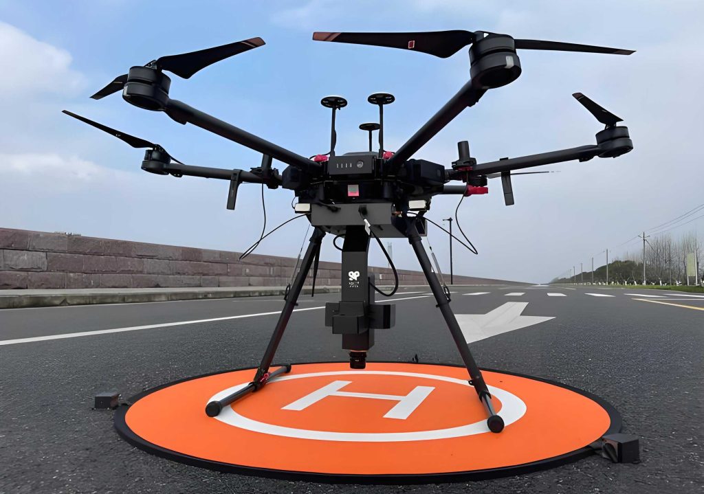
The operational scenario involves multiple potential takeoff and landing points within an urban area. From these, a subset is chosen as distribution centers (depots), while the remainder act as customer demand points. A fleet of heterogeneous, rechargeable multi-rotor UAV drone is deployed from these centers. Each UAV drone departs from its assigned center, delivers parcels to a sequence of customer points, and returns to the same center, completing a closed route. The problem is defined on a network represented by several sets: $N = \{1, 2, …, n\}$ is the set of all delivery nodes (including centers and demand points), $M = \{1, 2, …, m\}$ is the set of heterogeneous UAVs, and $K = \{1, 2, …, k\}$ is the set of selected distribution centers. Key assumptions include constant UAV cruise speed, each delivery task being performed exactly once by one UAV drone, and known, fixed expected and acceptable service time windows for each customer.
Multi-Objective Optimization Model Formulation
The core of the route planning problem is captured by a multi-objective mathematical model with three distinct goals.
Objective Functions
1. Minimize Total Weighted Flight Distance: This objective directly correlates with operational costs (e.g., energy consumption) and is fundamental for efficiency.
$$ \min f_1 = \sum_{i=1}^{m} \sum_{j=1}^{n} \sum_{r=1}^{n} \sum_{t=1}^{T} \alpha_i d_{jr} x_{ijr}^t $$
where $\alpha_i$ is the unit operating cost per distance for UAV drone $i$, $d_{jr}$ is the Euclidean distance between nodes $j$ and $r$, and $x_{ijr}^t$ is a binary variable equal to 1 if UAV drone $i$ flies from node $j$ to node $r$ in time period $t$.
2. Minimize Robust Total Flight Time: To ensure reliability against uncertainties like wind or service delays, we minimize the worst-case (maximum) mission completion time across all UAV drones. This enhances system robustness.
$$ \min f_2 = \max_{i \in M} \left\{ \sum_{j=1}^{n} \sum_{r=1}^{n} \sum_{t=1}^{T} \left( \frac{d_{jr}}{\theta_{jr} v_i} \right) x_{ijr}^t + \sum_{j=1}^{n} \sum_{t=1}^{T} \tau_{ij}^{\text{service}} x_{ijr}^t \right\} $$
Here, $v_i$ is the cruise speed of UAV drone $i$, $\theta_{jr} \in [0.8, 1.2]$ is a wind impact factor for the leg from $j$ to $r$, and $\tau_{ij}^{\text{service}}$ is the service time of UAV drone $i$ at node $j$.
3. Maximize Demand Satisfaction Rate: Prioritizing critical deliveries (e.g., medical supplies) is crucial. This objective maximizes the weighted sum of satisfied demand proportions.
$$ \max f_3 = \frac{ \sum_{j=1}^{n} \beta_j \left( \sum_{i=1}^{m} \sum_{t=1}^{T} \min(w_{ij}^t y_{ij}^t, D_j) \right) }{ \sum_{j=1}^{n} \beta_j D_j } $$
where $\beta_j$ is the priority weight of customer $j$, $y_{ij}^t$ is the proportion of demand at node $j$ satisfied by UAV drone $i$ in period $t$, $w_{ij}^t$ is the actual delivery amount, and $D_j$ is the total demand at node $j$. For algorithmic purposes, this is converted to a minimization problem: $\min \tilde{f}_3 = 1 – f_3$.
These three objectives address economy ($f_1$), temporal reliability ($f_2$), and service quality ($f_3$), covering the essential aspects of logistics delivery. They are interdependent and often conflicting, necessitating a multi-objective approach to find balanced solutions.
Constraints
The model incorporates several practical constraints:
1. Flow Balance: Ensures route continuity for each UAV drone.
$$ \sum_{r=1}^{n} x_{ijr}^t = \sum_{l=1}^{n} x_{ilj}^t \quad \forall i \in M, j \in N, t \in T $$
2. UAV Assignment to Centers: Each UAV drone is assigned to exactly one distribution center, and each center has a limited capacity.
$$ \sum_{k=1}^{K} z_{ik} = 1 \quad \forall i \in M $$
$$ \sum_{i=1}^{m} z_{ik} \le C_k \quad \forall k \in K $$
where $z_{ik}$ is 1 if UAV drone $i$ is assigned to center $k$, and $C_k$ is the capacity of center $k$.
3. Dynamic Payload Constraint: The total weight carried by a UAV drone after leaving a node cannot exceed its maximum capacity $W_i$.
$$ \sum_{j=1}^{n} w_{ij}^t \le W_i \sum_{j=1}^{n} \sum_{r=1}^{n} x_{ijr}^t \quad \forall i \in M, t \in T $$
4. Robust Range Constraint: The total distance flown by a UAV drone in a mission must not exceed its maximum range $R_i$, considering the worst-case wind factor.
$$ \sum_{j=1}^{n} \sum_{r=1}^{n} \sum_{t=1}^{T} \frac{d_{jr}}{\theta_{jr}} x_{ijr}^t \le R_i \quad \forall i \in M $$
5. Time Window Constraint: The arrival time at a customer must fall within its acceptable time window $[E_j, L_j]$.
$$ E_j \le \tau_{ij}^{\text{arr}} \le L_j \quad \forall i \in M, j \in N $$
6. Composite No-Fly Zone Avoidance: The flight path $p(j, r)$ between any two nodes must avoid all defined no-fly zones $\omega_l$.
$$ p(j, r) \cap \left( \bigcup_{l=1}^{L} \omega_l \right) = \emptyset \quad \forall j, r \in N \text{ where } \exists x_{ijr}^t = 1 $$
7. Demand Satisfaction Constraints: Limit delivered amounts to actual demand and link delivery to visitation.
$$ \sum_{i=1}^{m} \sum_{t=1}^{T} w_{ij}^t y_{ij}^t \le D_j \quad \forall j \in N $$
$$ y_{ij}^t \le \sum_{r=1}^{n} x_{ijr}^t \quad \forall i \in M, j \in N, t \in T $$
Distribution Center Selection via Greedy Strategy
Selecting optimal locations for distribution centers from candidate sites is a precursor to route planning. A greedy strategy based on geometric coverage and dispersion is employed. Given $m$ centers to select from $n$ candidate points:
- Compute Geometric Center: Find the centroid $c$ of all candidate locations $l_i$.
$$ c = \frac{1}{n} \sum_{i=1}^{n} l_i $$ - Select First Center: Choose the candidate point closest to the geometric center as the first distribution center $c_1$.
$$ c_1 = \arg \min_{i \in \{1,…,n\}} d(l_i, c) $$ - Select Subsequent Centers: For selecting the $j$-th center ($j > 1$), choose the candidate point that maximizes the minimum distance to any already selected center. This promotes dispersion for better area coverage.
$$ c_j = \arg \max_{i \notin \{c_1,…,c_{j-1}\}} \left\{ \min_{k \in \{1,…,j-1\}} d(l_i, c_k) \right\} $$
The process repeats until $m$ centers are selected.
Improved NSGA-II Algorithm Design
The NSGA-II is well-suited for multi-objective optimization due to its mechanisms for maintaining population diversity and converging towards the Pareto front. Several enhancements are made to tailor it to the UAV drone delivery problem.
Chromosome Encoding
A composite chromosome structure $X = \{\text{DC}, \text{UA}, \text{R}\}$ is used:
- DC: Vector listing the selected distribution center IDs, e.g., $\{3, 7, 12, 19\}$.
- UA (UAV Assignment): Vector of length $m$ where the $i$-th element indicates the center ID to which UAV drone $i$ is assigned.
- R (Routes): A set of $m$ routes. Each route $r_i$ is a sequence starting and ending at the assigned center ID, e.g., $\{k, j_1, j_2, …, k\}$.
Multi-Strategy Population Initialization
To enhance initial diversity, four strategies are cyclically used during population generation:
- Payload-Priority: Sort UAV drones by descending payload capacity. Assign tasks first to UAVs with higher capacity.
- Range-Priority: Sort UAV drones by descending maximum range. Prioritize UAV drones with longer endurance.
- Balanced Strategy: Sort UAV drones by a composite score $s_i = \frac{f_{\text{cap},i} \cdot f_{\text{range},i}}{f_{\text{cost},i}}$, where $f_{\text{cap}}$ is payload, $f_{\text{range}}$ is range, and $f_{\text{cost}}$ is unit cost.
- Random Strategy: Generate individuals randomly to preserve diversity.
Fitness Evaluation, Non-dominated Sorting, and Crowding Distance
The fitness vector for an individual $X$ is $F(X) = [f_1(X), f_2(X), \tilde{f}_3(X)]$. Non-dominated sorting ranks individuals into Pareto fronts. For individuals on the same front, crowding distance $CD_i$ measures the density of solutions around it, promoting diversity:
$$ CD_i = \sum_{m=1}^{3} \frac{f_m(i+1) – f_m(i-1)}{f_m^{\max} – f_m^{\min}} $$
where $f_m(i+1)$ and $f_m(i-1)$ are the objective values of the neighboring solutions after sorting by objective $m$.
Selection, Crossover, and Mutation
Selection: A tournament selection based on front rank and crowding distance is used. Additionally, individuals failing a minimum demand satisfaction rate threshold (e.g., 85%) are filtered out to focus the search on feasible solutions.
Crossover: A multi-point crossover operator is applied separately to the DC, UA, and R parts of the chromosome with different probabilities (e.g., 0.4, 0.4, 0.2).
Adaptive Mutation: Mutation probabilities are set for different actions: replacing a distribution center (prob. 0.3), reassigning a UAV drone to a different center (prob. 0.3), and performing local path optimization like swapping two nodes in a route (prob. 0.4). If the algorithm stagnates, mutation rates are adaptively increased to escape local optima.
Algorithm Flow
- Initialize: Generate initial population $P_0$ using multi-strategy initialization.
- Main Loop (for generation $g = 1$ to $G_{\max}$):
- Evaluate objective values for all individuals in $P_g$.
- Filter solutions based on the minimum demand satisfaction rate.
- Perform non-dominated sorting and calculate crowding distance for the filtered population.
- Generate offspring population $Q_g$ via selection, crossover, and mutation.
- Combine parent and offspring: $R_g = P_g \cup Q_g$.
- Perform environmental selection on $R_g$ based on non-domination rank and crowding distance to form the next generation $P_{g+1}$.
- Output: Return the non-dominated solutions from the final population as the Pareto-optimal set.
Simulation Experiments and Analysis
Parameter Settings
The simulation environment is a 20 km × 20 km urban area with 40 candidate takeoff/landing points. The greedy strategy selects $k=4$ distribution centers. Each center has a maximum capacity of 7 UAV drones, with a total heterogeneous fleet of $m=20$ UAV drones available. Their parameters vary, as exemplified below:
| UAV Drone ID | Max Speed (km/h) | Range, $R_i$ (km) | Payload, $W_i$ (kg) | Unit Cost, $\alpha_i$ ($/km/kg) |
|---|---|---|---|---|
| UAV1 | 60 | 25 | 8 | 0.120 |
| UAV2 | 65 | 30 | 10 | 0.110 |
| UAV3 | 70 | 35 | 12 | 0.100 |
| … | … | … | … | … |
| UAV18 | 92 | 60 | 24 | 0.050 |
| UAV19 | 95 | 65 | 25 | 0.045 |
| UAV20 | 100 | 70 | 28 | 0.040 |
NSGA-II parameters: population size = 120, maximum generations = 150, crossover probability = 0.90, mutation probability = 0.25, tournament size = 3, minimum demand satisfaction rate threshold = 0.85.
Results and Discussion
1. Validity of Pareto Solutions
The algorithm successfully generates a well-distributed set of Pareto-optimal solutions. The 3D Pareto frontier clearly shows the trade-off relationship between the three objectives. Analysis of the correlation between objective pairs (e.g., distance vs. time) reveals coefficients like 0.777, indicating related but non-substitutable goals, validating the multi-objective approach.
Specific solutions highlight the trade-offs. For instance:
- Distance-Optimal Solution: Achieves the shortest total flight distance (e.g., 160.53 km) but may have a lower demand satisfaction rate (85.8%) and use fewer UAV drones, potentially leaving some customers unserved.
- Time-Optimal Solution: Achieves the shortest robust mission time (e.g., 14.81 min) but often at the cost of an even lower service rate (85.4%).
- Satisfaction-Optimal Solution: Achieves 100% demand satisfaction but requires a longer total distance (226.44 km), more time (23.48 min), and possibly more UAV drones.
The Pareto set provides various balanced solutions between these extremes, allowing the operator to choose based on current priorities (cost, urgency, or service level).
2. Algorithm Efficiency
The computational efficiency of the improved NSGA-II is tested by scaling the number of delivery points. The results, shown below, indicate that the algorithm remains computationally feasible for moderate-scale problems.
| Number of Delivery Points | Total Execution Time (s) | Average Time per Generation (s) | Algorithm Efficiency (Generations/s) |
|---|---|---|---|
| 40 | 103.00 | 0.687 | 1.46 |
| 50 | 126.17 | 0.841 | 1.19 |
| 60 | 157.74 | 1.052 | 0.95 |
| 70 | 181.73 | 1.216 | 0.86 |
As the number of points increases, resource bottlenecks appear. With 60 points, the maximum achievable satisfaction rate drops from 100% to around 92.2%, indicating that the fixed fleet of 20 UAV drones becomes insufficient. At 80 points, no feasible solution is found, suggesting a need to increase the number of UAV drones or distribution centers for larger-scale operations.
3. Impact of UAV Drone Fleet Size
Constraining the maximum number of UAV drones that can be used significantly impacts the Pareto frontier. Tightening the constraint from “no limit” (effectively 11 drones used by best solutions) to a maximum of 9 drones causes the frontier to contract. Interestingly, under the 9-drone constraint, the algorithm discovers solutions with even shorter minimum flight distances (146.28 km vs. 160.53 km), demonstrating that resource constraints can force more efficient route consolidation. However, the demand satisfaction rate inevitably suffers. The number of UAV drones is a critical resource parameter, and identifying its lower feasible bound (e.g., 9 drones for the 40-point, 4-center scenario) is essential for practical deployment planning.
Conclusion
This paper addresses the complex problem of logistics UAV drone delivery route planning through a comprehensive multi-objective optimization framework. The proposed model effectively captures the essential trade-offs between economic cost (flight distance), delivery reliability (robust time), and service quality (demand satisfaction rate). The improved NSGA-II algorithm, with its tailored chromosome encoding, multi-strategy initialization, and adaptive operators, proves effective in generating a diverse set of high-quality Pareto-optimal solutions. The integration of a greedy strategy for distribution center selection provides a practical method for initial network setup. Simulation results confirm that the three objectives are non-substitutable and that the multi-objective approach is necessary. The analysis also highlights the critical influence of key resources, particularly the number of UAV drones and distribution centers, on feasible solution spaces. This work provides a solid methodological foundation for decision-support systems in UAV-based logistics, enabling operators to select route plans that best align with their specific operational priorities and resource constraints. Future work may involve dynamic re-planning with real-time information, incorporation of more sophisticated energy consumption models, and testing in larger, more complex urban networks.